Setting up RStudio for success

This page provides an overview for setting up and working in RStudio that will set you up for success in creating a reproducible workflow for data analysis in R.

What are R and RStudio?

It is important to clearly distinguish between R and RStudio because they can easily become intertwined. In short:

• R is the programming language
• RStudio is the application in which we will write and run R code. It is the integrated developer environment (IDE) most closely associated with R.

It is possible to run R in many different applications and environments. In fact, Posit, the company behind RStudio is currently building a new IDE for data analysis called Positron. You can also run R on the command line or in another IDE such as Visual Studio Code.

Figure 1: An R session running in the Terminal app.

We will use RStudio because it is a mature, open source application that provides many features that helps people write good R code and is closely integrated with Quarto. It is also the most widely used IDE for R.

Navigating RStudio

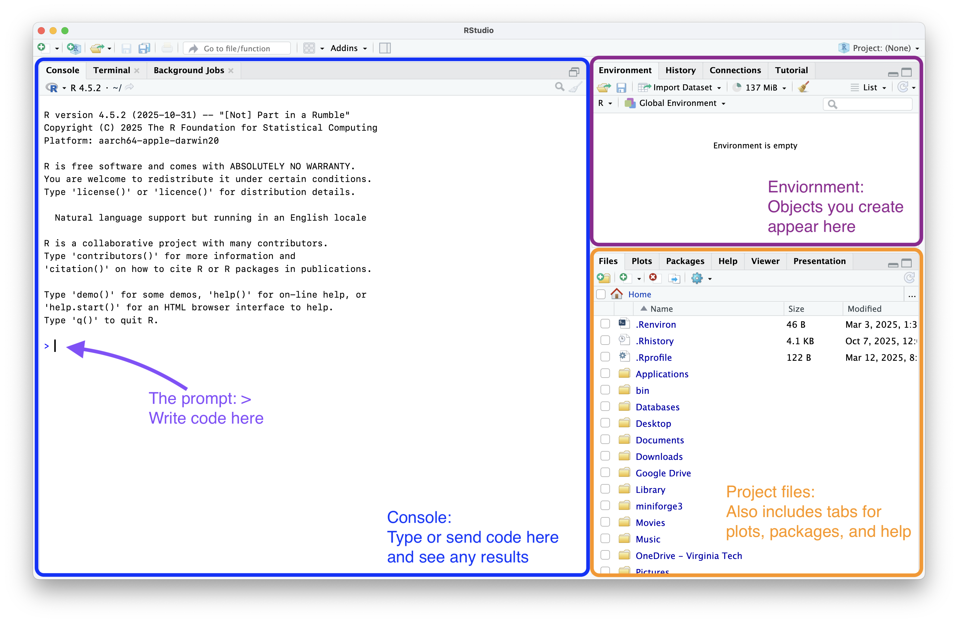
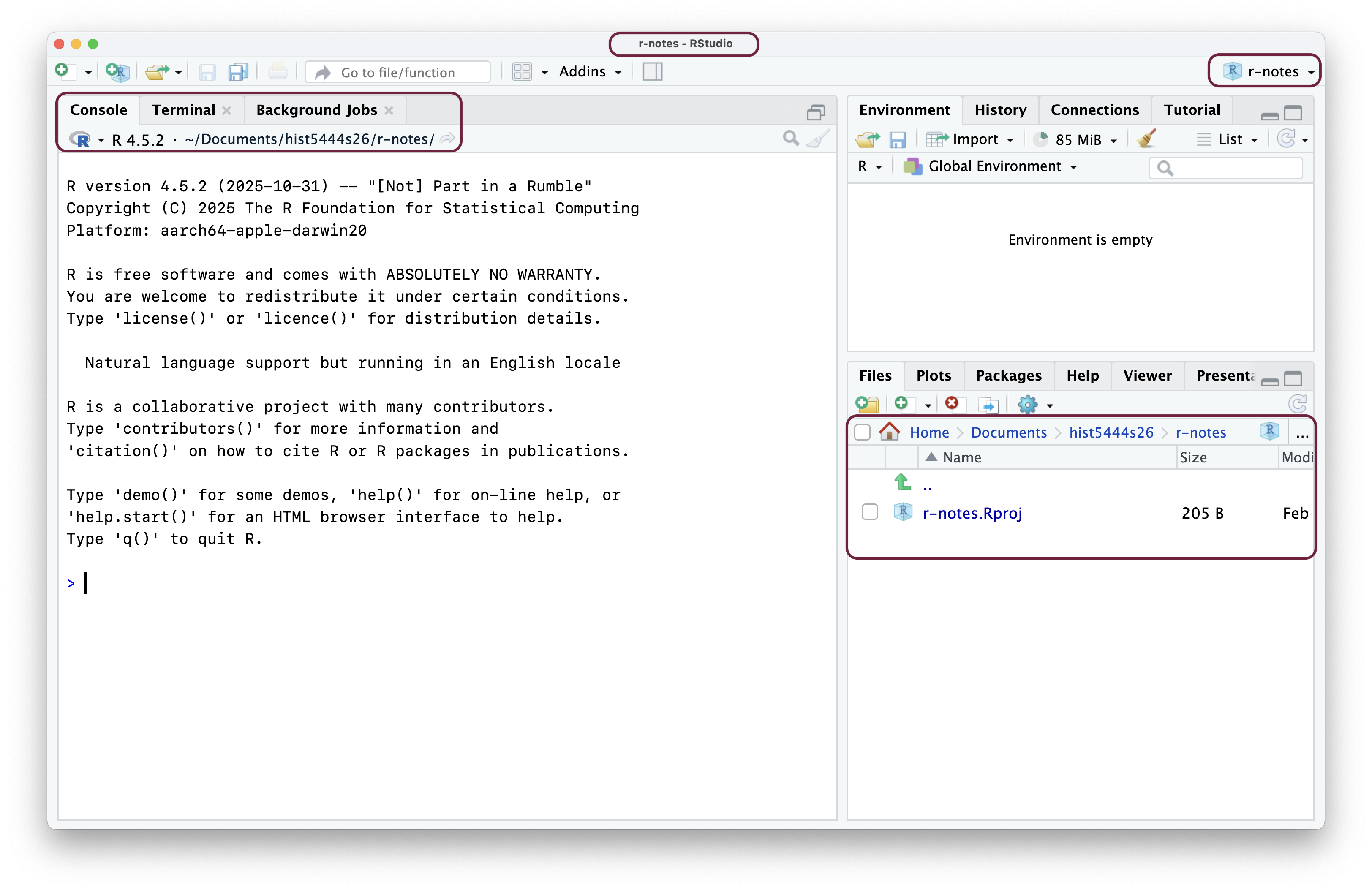
When you open up RStudio for the first time you will be presented with a three panel view:

• The left panel is the console. This is where you write or send code, run it, and see any output. You type your code after the prompt, which in R is >.
• The upper-right panel shows any objects you create in your session.
• The bottom-right panel shows your project files but also has tabs to show plots you make, packages you have installed, and a viewer for documentation.

Figure 2: RStudio at startup with three panels: console, environment, and files.

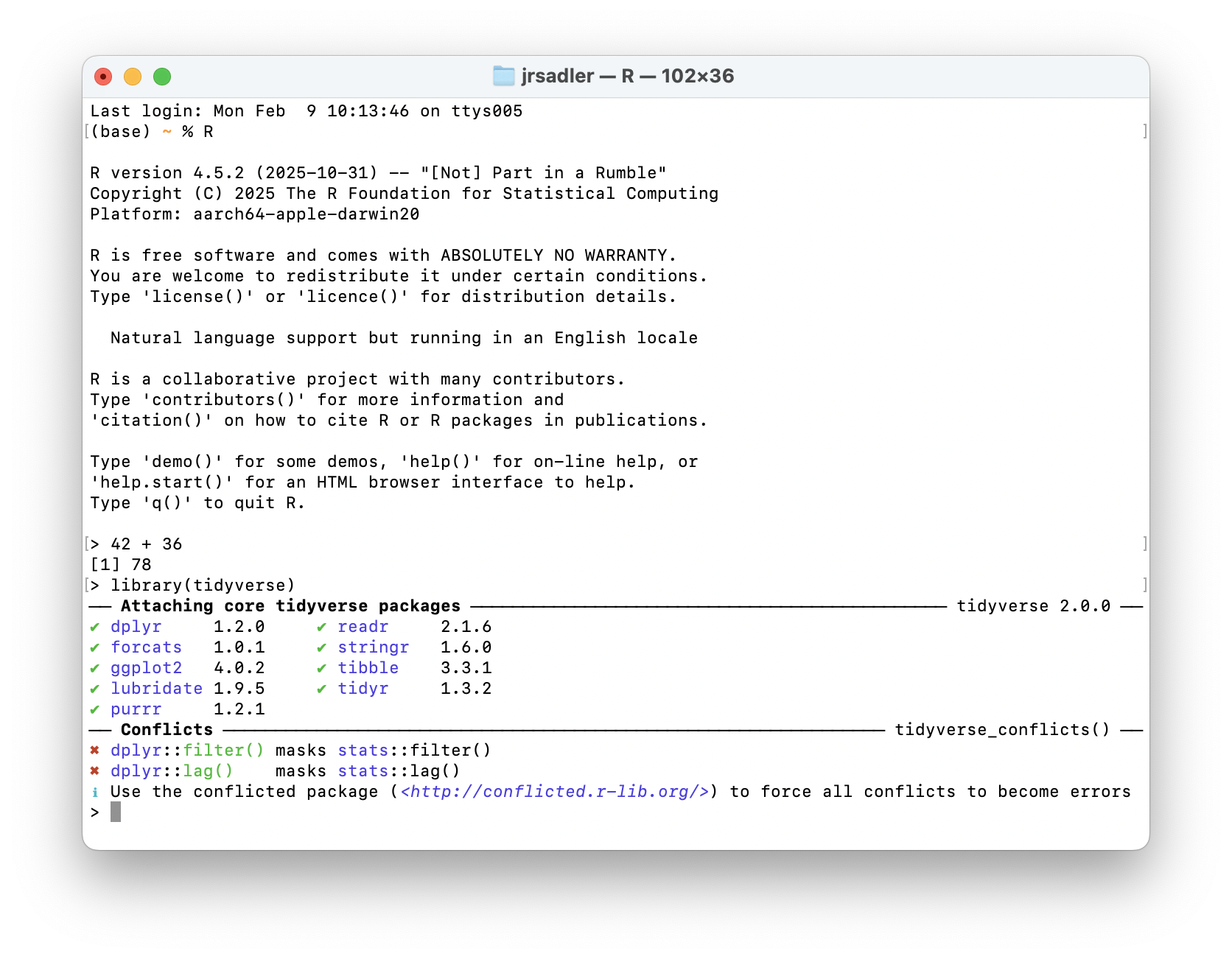
Type in your first R command to make sure everything is working. Type out a mathematical calculation and press Return or Enter to run the line of code.

RStudio projects

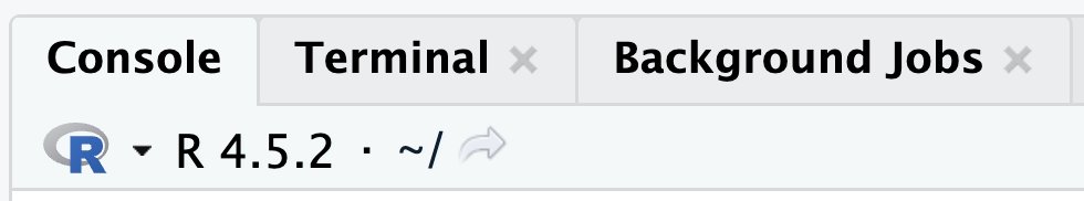
One of the foundational features of RStudio is the concept of projects. Projects set up your analyses for reproducibility by making it clear where your analysis lives and how your data, scripts, and all other files that belong to an analysis are related to each other. In short, they are all contained in a project folder. Projects are based on R’s notion of the working directory. This is the folder where R starts when you ask it to load data files or save scripts. If this is the first time that you have opened RStudio, your working directory is probably your home directory. On macOS this is represented with ~/, on Windows likely with C:\Users\[your-username]. You can see this at the top of the console panel.

Figure 3: Current working directory.

RStudio projects provide a clear and explicit way to tell R where to start (to set your working directory) and keep all of your analysis together. Let’s create our first project. This project will hold all of the code and data we will work on in our in-class sessions. When you want to work on a project with your own data, follow these steps again to create a new project in a different folder.

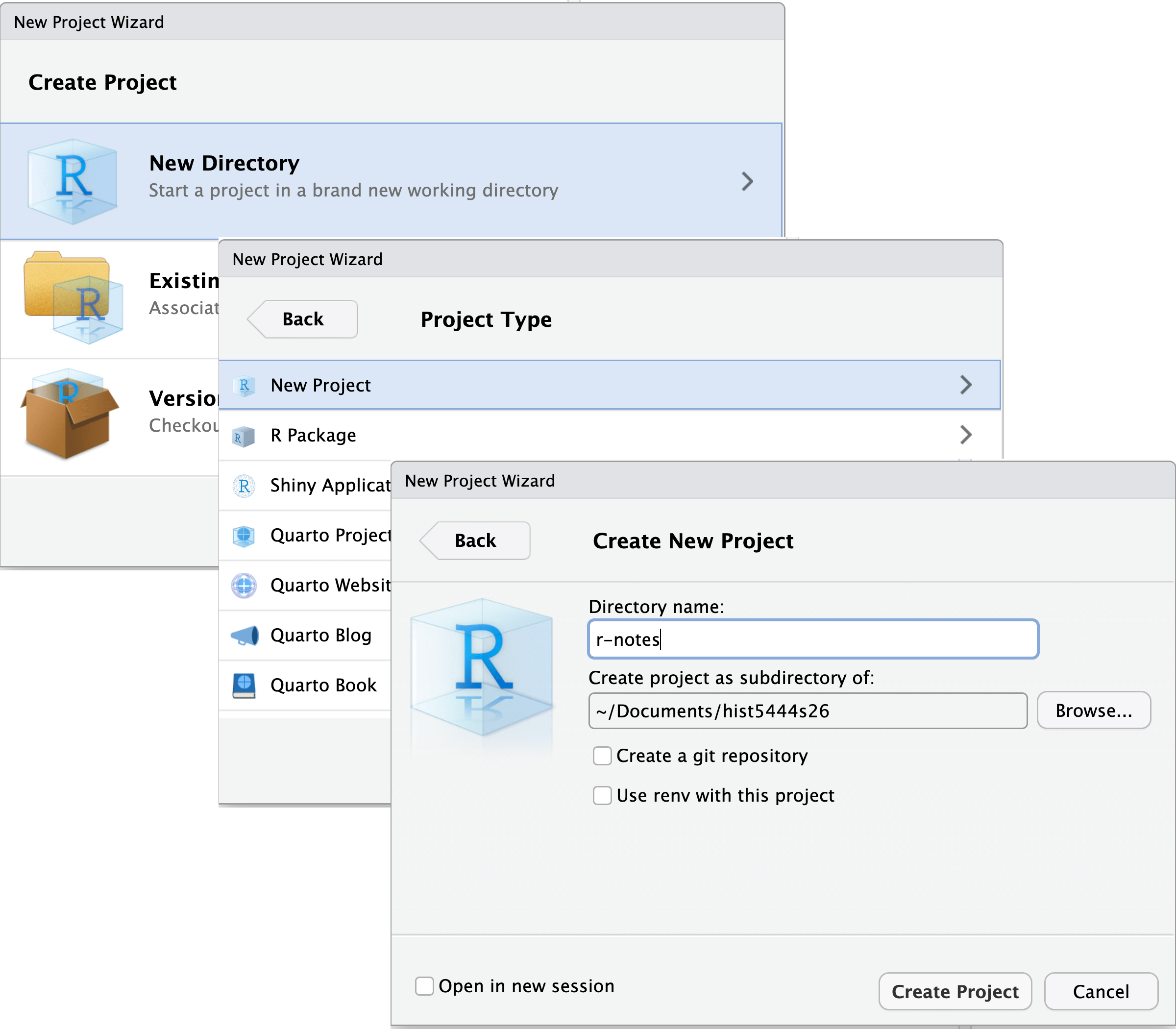
1. Go to the File menu and select New Project…
2. In the New Project Wizard select New Directory.
3. Choose New Project for the Project type.
4. Name your project and choose where to put it.
   • For this first project under Directory name we will use r-notes.
   • Then, select Browse… to put the project folder inside your hist5444s26 folder that contains the work done for this course. If you have not created this folder yet, do so now in Finder or File Explorer.
   • Finally, select Create Project

Figure 4: Steps to create a project: (top) select New Directory, (middle) choose New Project for the project type, (bottom) choose what to name the project and where to put it.

RStudio will start back up but now your working directory will be the new project folder you created, in this instance r-notes. You can verify you are in your new project in four different locations in the RStudio interface.

1. The name of the RStudio window will now contain r-notes.
2. The top of the has the path on your computer from your home to the project folder. For me it is ~/Documents/hist5444s26/r-notes.
3. The project dropdown on the top-right of the RStudio window. You can use this menu to quickly switch between different projects.
4. The files panel will show the path to your working directory and a single file named r-notes.Rproj.

Figure 5: RStudio project interface, highlighting areas that show the current project.

Setting up your project structure

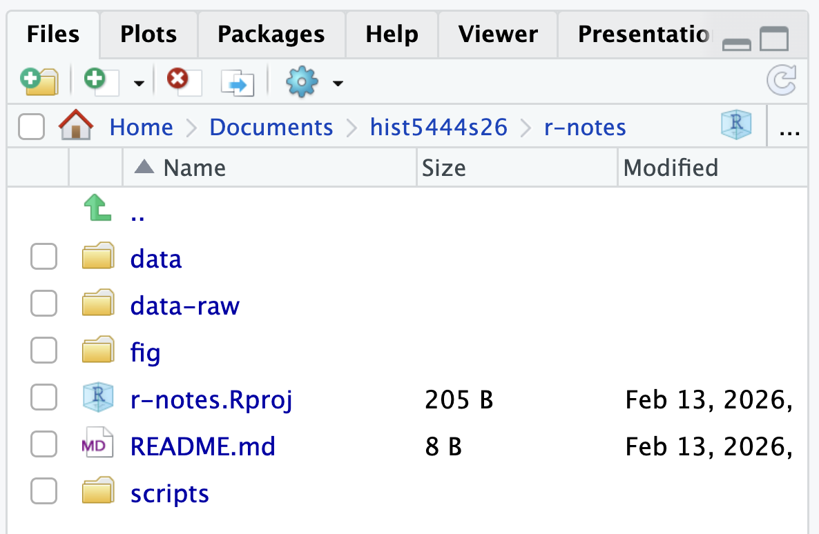
Let’s finish setting up the new project by providing some structure, adding folders to separate our raw data, any modified data we create, our scripts we write, and the figures we make. The most important aspect of this is to separate our raw data from our modified data we create using R.¹ Keeping these two types of data separate will protect you from making errors and possible data loss. You can add the folders in the RStudio files panel by clicking ojn the folder with the plus sign, or you can create the folders in Finder or File Explorer. Your folders should be named:

• data/: Any modified data that you want to store after cleaning or analyzing your raw data.
• data-raw/: Raw data that you have created or gotten from an external source.
• scripts/: Where you will keep your R scripts and any other documents such as Quarto documents.
• fig/: A place to store any visualizations you make in the course of your analysis.
• README.md: Lastly you can create a README file to explain the purpose and structure of the project. To create a new Markdown file in RStudio go to File -> New File -> Markdown File.

Figure 6: Project folders.

TipWhat is the r-notes.Rproj file?

The r-notes.Rproj file is a plain text file that has a couple of project based settings in it. You can click on it in RStudio and it will open a dialogue window. Generally, you do not want to touch the file. Primarily, the file projects the best target for opening up your project. Double-click on any .Rproj file and RStudio will open to that project.

NoteRelative vs absolute paths

Projects enable you to access files such as data with relative paths from your working directory. Within our r-notes project we can access a data file called SAFI_clean.csv using the relative path: data-raw/SAFI_clean.csv.

If we did not use projects and kept our working directory as our home directory, we would have to use absolute paths. Absolute paths point to a file or folder regardless of the working directory. On my computer it would be ~/Documents/hist5444s26/r-notes/data-raw/SAFI_clean.csv. This might work for those on a Mac because we were specific about naming our folders, but it will not work on Windows.

If you were to move the r-notes folder into another folder, absolute paths would not even work on your computer any more. However, if you give your r-notes folder to someone else and you use projects and relative paths, the paths will correctly find the data on their computer.

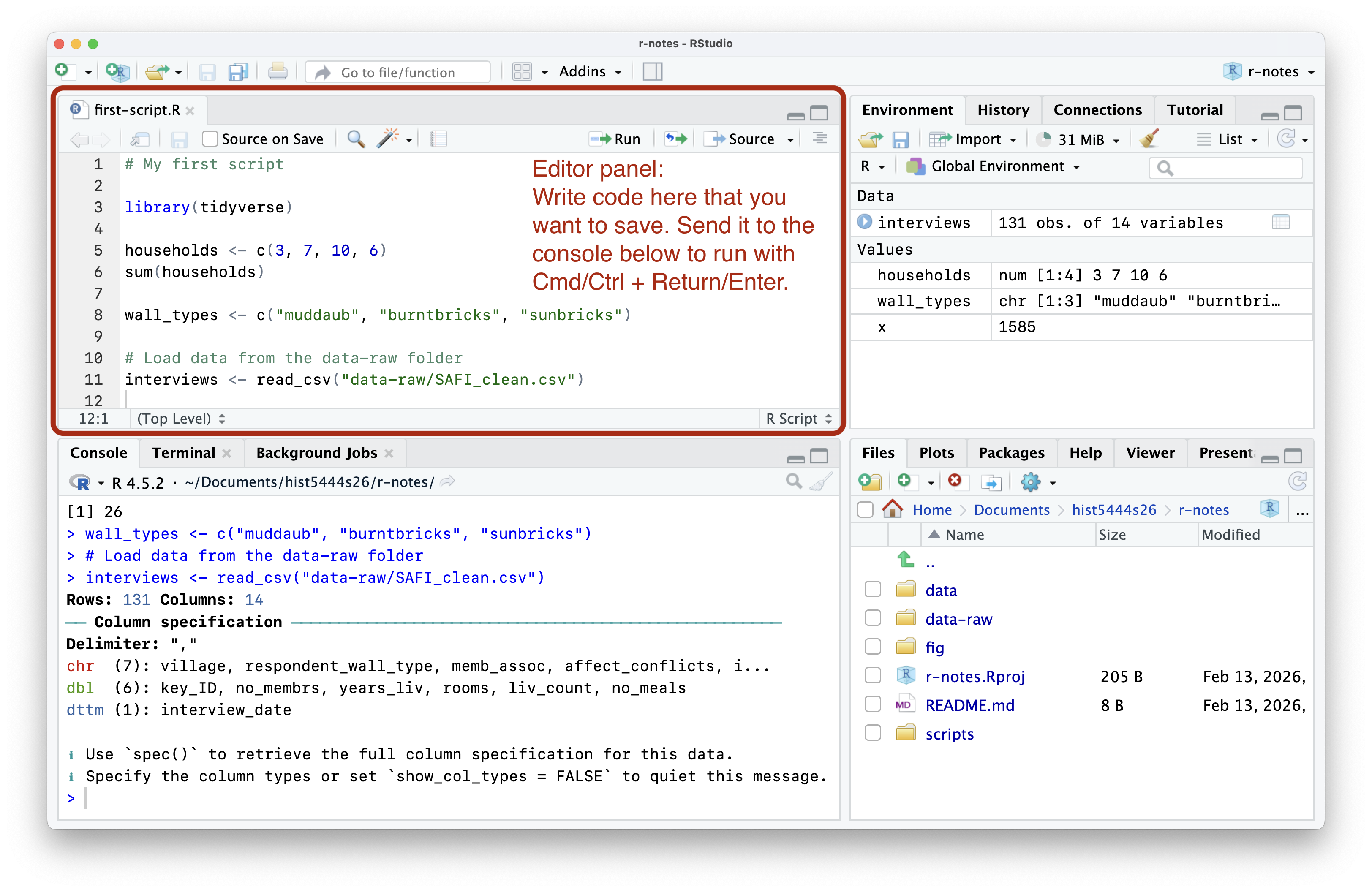
The editor panel

Now that you have created a project, we can create our first R script where we will save our code. When you create a new R script or any other type of file, a fourth panel will appear in the upper right and the console will shrink to the bottom-right position. You can create a new R script (this is a text file that ends with the extension .R) in many ways.

• Go to File -> New File -> R Script
• Click on the plus sign with the blank paper behind it in the upper-left corner of RStudio and select R Script.
• Similarly, click on the plus sign with the blank paper behind it in the upper-left corner of the Files panel.
• Or with a keyboard shortcut: Cmd/Ctrl + Shift + N.

Figure 7: RStudio with all four panels: editor, console, environment, and files.

The workflow

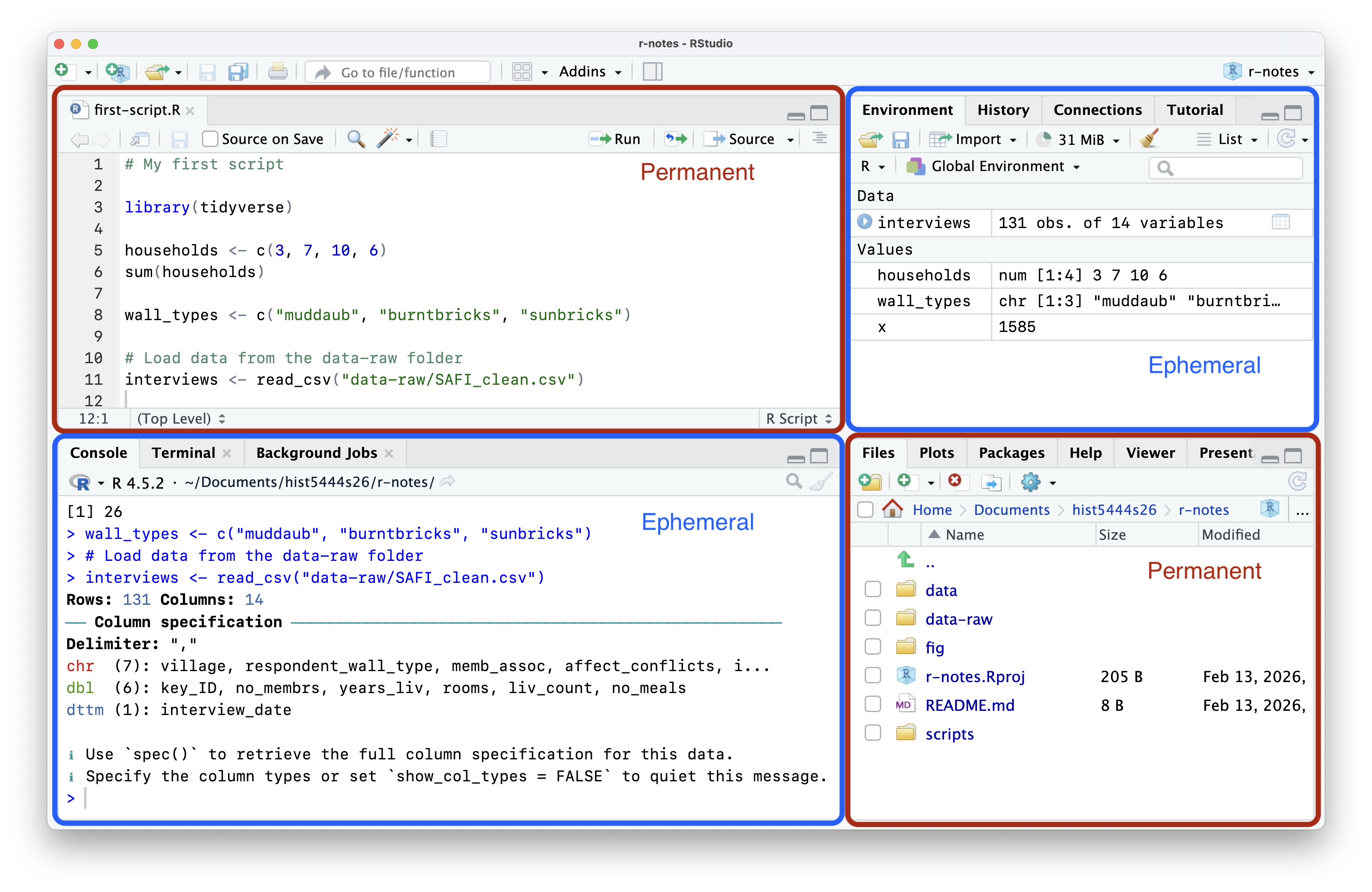
The basic workflow for RStudio is to work on writing and running code in the left two panels and inspect aspects of what you are doing or what you have created in the right two panels.² Let’s concentrate on the two panels on the left.

The console can be thought of as where the action happens. It is where code is actually run and where any outputs will be printed. However, the console is also ephemeral. You run code expression by expression, pushing each line of code further and further up into the console’s history, out of sight and out of mind. You can look at your history, but, practically speaking, there is no good, clear way to track what you have done just by using the console.

This is where the editor panel comes in. The editor panel shows text documents in which you will save the code and any documentation or explanations that you want to save. We will primarily be working with R scripts and Quarto documents in this course. Here, we will stick to R scripts.

Scripts and reproducibility

Scripts are at the foundation of reproducibility. They contain the code that performed a certain set of analysis or created a visualization that can be run by you or someone else later. Unlike the console, scripts are meant to be permanent or at least record what you have done. You save scripts, but you do not save what happened in the console.³

An R script is a plain text document in which everything that is typed is assumed to be R code that will be sent to the console. To run code from a script (or send it to the console) you cannot just type Return/Enter. That moves you to the next line. Instead, place your cursor anywhere within an R expression and press Cmd + Return or Ctrl + Enter. If you want to write comments in a script to take notes or tell future you or any collaborators why you did something, you need to place a hashtag # before it. Anything after # will not be run as code.

• Execute an R expression from a script: place cursor within the expression and press Cmd + Return or Ctrl + Enter
• Comment: #

Try it out for yourself.

This distinction between permanent and ephemeral also translates to the panels on the right. The files pane (bottom right) shows the scripts you create and any data or visualization you save. These are permanent. The environment panel shows the objects created in a session by running code in the console. These objects are ephemeral. They exist and can be used in this session, but they can always be recreated from the script.

The script trumps the environment panel; it is the source of truth. The code that creates the object is much more important than the object itself. Think of it this way, if you have it right in the environment but wrong in a script, it will not do you much good when you come back to your code after a break and find that things are out of whack.

Figure 8: The editor and files panels are the primary sources of truth. The console and environment panels represent the ephemeral objects created in a session.

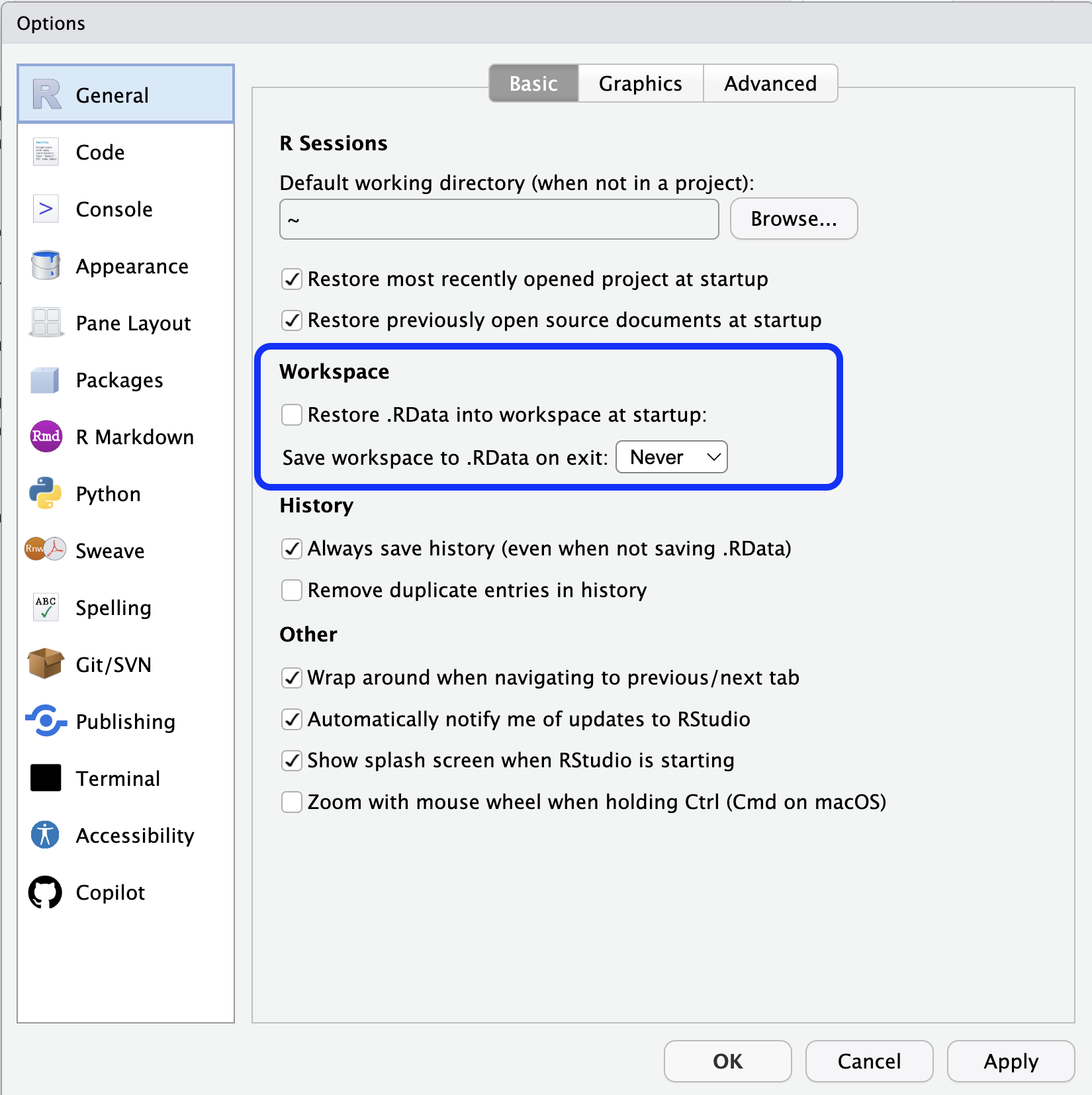
Setting up RStudio for reproducibility

We need to make some important changes to the default settings in RStudio to ensure that R scripts remain the source of truth of your analysis not your environment. Go to Tools -> Global Options and uncheck Restore .RData into workspace at startup and set Save workspace to .RData on exit to Never.

Figure 9: RStudio Global Options: Set these options for the Workspace.

Let’s see what this does. Make sure that you have created objects in your environment. Then, restart your session. You can do this by going to the Session menu -> Restart R. Your environment panel should be empty now. This might seem like it is painful, but it is short-term pain for long-term gain. It will teach you to keep what you want to save in your R script so that you can always recreate objects or rerun analysis later.

In fact, running Restart R and then running your script, either one line at a time (hit Cmd + Return or Ctrl + Enter over and over) or Cmd/Ctrl + Shift + S to re-run the entire script, is a good way to ensure that your script is correct. Better to find out now if there is a problem than weeks or months down the road.

Packages

After getting RStudio set up, the next step is to install the main packages we will use in the course. R comes with a preinstalled set of packages known as base R. The real power of R comes from combining this strong foundation for data analysis with other packages built by community members. Generally you will install packages through the central package repository called CRAN (The Comprehensive R Archive Network), which is also where you downloaded R. There are over 23,000 packages on CRAN.⁴

Installing packages

Most importantly for this class, we need to install the tidyverse set of packages. There are two ways to do this. Either through a function on the console or using the RStudio GUI (Graphical User Interface). I generally prefer to use the console.

1. You can install packages with the install.packages() function with the names of the packages you want to install in a character vector. Let’s start by just installing the tidyverse package.

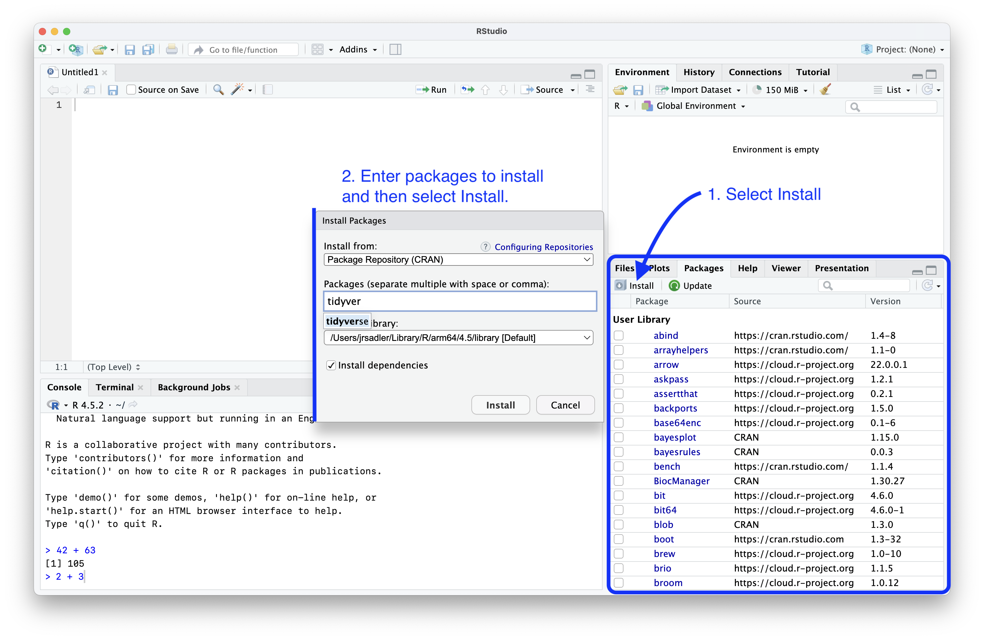
install.packages("tidyverse")

2. To use the graphical interface to install packages:
   • Select the Packages tab in the Files panel on the bottom right of RStudio.
   • Click on Install button on the top left of the panel.
   • This will open a popup dialogue. Type in the packages you want to install—in this case tidyverse—and then click Install.
   • Note that RStudio will actually run the command install.packages("tidyverse") in the console.

Figure 10: Installing packages with the Packages panel in RStudio.

Using packages

The tidyverse set of packages is now installed, but to actually use the functions from the package in an R session you need to load the package. This is done with library(). Try it for yourself.

library(tidyverse)

You do not need to put quotation marks around tidyverse because the library() function knows where to look for something called tidyverse. You can put quotation marks around it if you want to. You should get an output in your console that looks like this:

Figure 11: Output from loading the tidyverse, showing the packages loaded and functions that conflict with those from other packages.

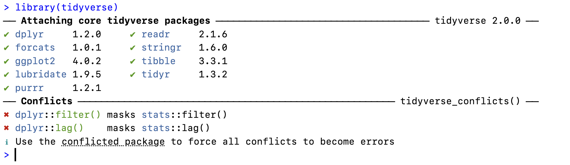
You see a list of the nine core tidyverse packages and their versions: dplyr, forcats, ggplot2, lubridate, purrr, readr, stringr, tibble, tidyr. You will also see a message that there are conflicts. This sounds scary but is expected behavior. This message tells us that dplyr has functions called filter() and lag(), which are also names for functions in base R. When you use these function after loading the tidyverse, you will use the dplyr version, which is what we want.

Remember, because we set up RStudio for reproducibility, you need to run library(tidyverse) every time you begin a new session. Therefore, you should load the packages you will use at the start of your script. Writing library(tidyverse) at the top of each script is a good practice to begin with.

Updating packages

Packages are often changing, fixing bugs (and adding some) and bringing new features so it is a good idea to update your packages every once in a while.⁵ Again, there is a way to do this in the console and through the Packages panel.

1. Run update.packages() and choose y to update the packages.
2. To use the graphical interface to update packages:
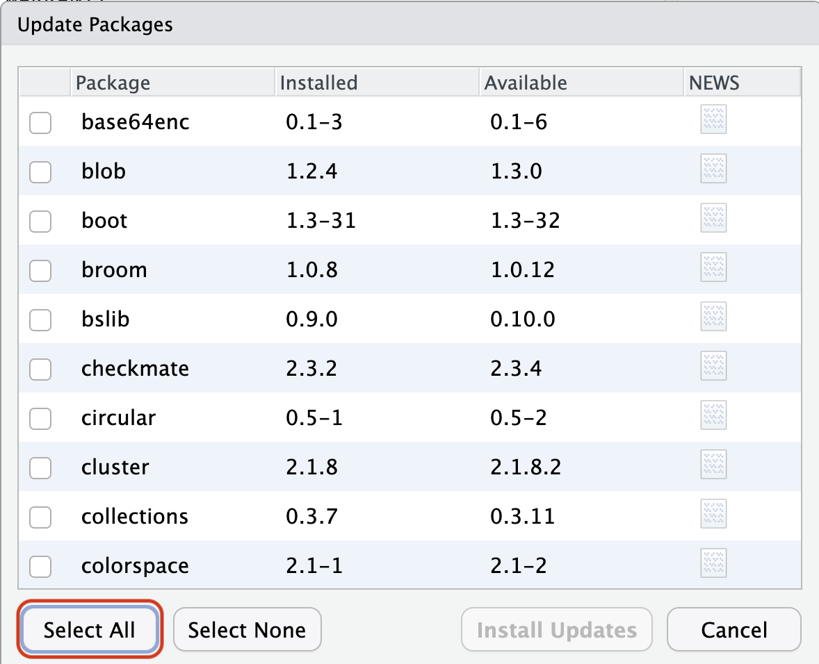
   • Click on Update button on the top left of the Packages tab of the Files panel. It is right next to Install.
   • You can click the Select All button on the bottom right of the dialogue window that pops up.
   • Then Install Updates.

Figure 12: Updating packages with the Packages panel in RStudio.

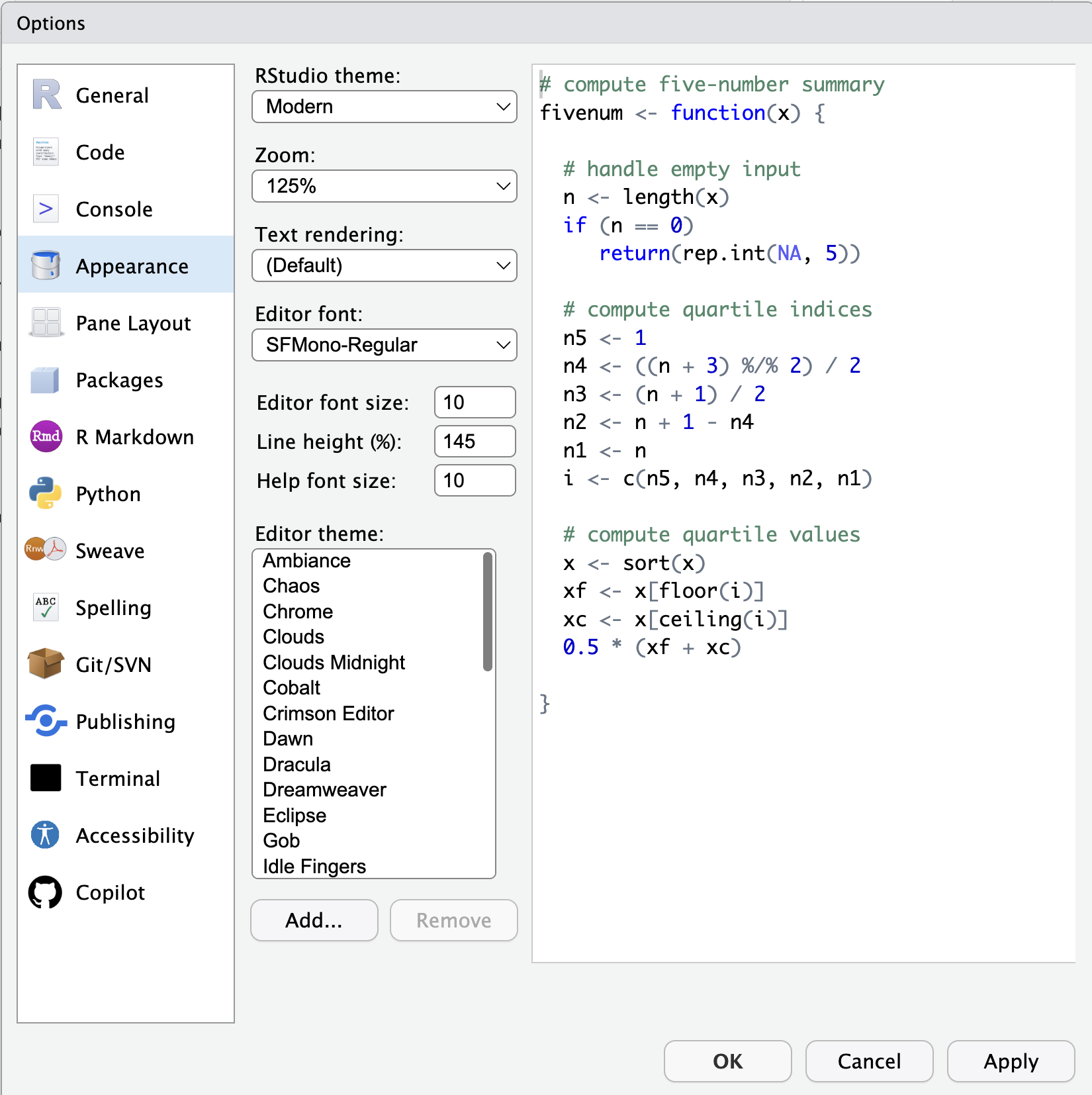
Other tweaks

There are also a couple of tweaks that you can make to the appearance and way things work in RStudio that might be worth your time. The settings for RStudio are found under Tools -> Global Options. Under the Appearance tab you can change the color theme for RStudio, choose your font and font size.

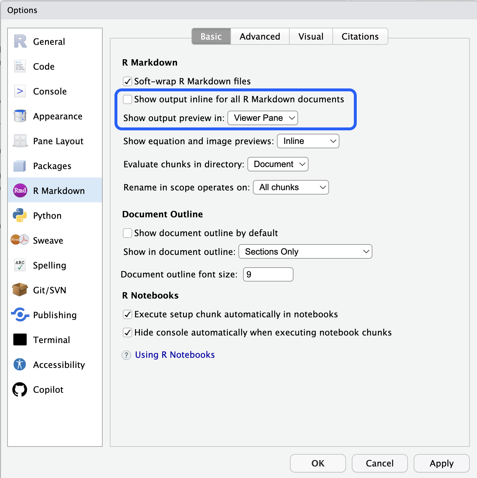
Another change that I like to make is in the R Markdown tab. This changes the settings for notebook-like files such as R Markdown and Quarto. I like to uncheck Show output inline for all R Markdown documents. This makes Quarto documents act more like scripts. Instead of printing output below a cell block and in the console, the output only goes to the console.

Figure 13: Change the color scheme, font, and font size of RStudio in the Appearance settings.

Figure 14: You may want to uncheck Show output inline for all R Markdown documents.

The Code tab has a couple of settings that you might want to change.

• I suggest using the native pipe operator (|>) by checking the box.
• Under Display you might want to uncheck Show margin. This will turn off the vertical line in the editor pane.
• At the bottom of Display there is a check box for rainbow parentheses. This turns each set of parentheses a different color, which can help you keep track of where you are in more complex code.

Play around with the themes to make RStudio a nice, fun place to be. You might even look for some different monospaced fonts.⁶

Footnotes

1. Raw data may be an oxymoron, but it is a useful one when setting up our projects.

2. You can move the panels around in Tools -> Global Options if you want to.

3. This is largely true if a bit overdramatic. The History tab shows the code expressions you have run.

4. You can also install packages from other repositories such as R Universe or on GitHub, but we will not need to do that for this course. The process for installing from these other places is similar.

5. How often is up to you. Packages are generally stable, so I find there is usually little downside to updating. I update packages once a week but once a month would be plenty frequent.

6. Some free monospaced fonts that you might check out are Apple’s SF Mono, Fira Code, Hack, Source Code Pro, and Iosevka.