library(tidyverse)
library(tidygeocoder)
library(sf, verbose = FALSE)
library(rnaturalearth)Putting maps on your website
The problem
When making a map, we often need to download the data using an R package. This could be data for the base map from rnaturalearth, more detailed street and location data from Open Street Maps using osmdata, or locations that we geocode with tidygeocoder. We want to do this active downloading as few times as possible. We want to download the data, make sure that it is correct and maybe clean it up, and then save the data for future usage. This guide will show how to do that.
The solution
The solution is to break up the steps of making a map into separate scripts. We get and prep the data once. Then we can use the data to make as many maps as we want. This is good practice for thinking about how we should be dividing up scripts and when to save data compared to when we can recreate it through our R scripts.
There are two basic ways to do this:
- Use an R script within the website project folder to download and clean the data. An R script (named something like
map-data.R) will not be rendered in the website by Quarto. - Download the data and potentially make the map in a separate RStudio project. You can either create the map in that project, save an image file, and then use the image on your website, or you can copy over the cleaned data files to website project to work on them there.
Either way you decide to structure your project, there are four basic steps to follow:
- Download the data.
- Check that the data is correct and clean it up.
- Save the data; write it out to a
data/folder. - Read in the data when you want to make a map.
Let’s show how to do this for two different kinds of geographic data we will want to download from the internet: geocoded data and base map data.
First we load the packages we are going to use.
Geocoded data
Geocoding location data is something that we want to do once, make sure that it is correct, and then save the resulting data. It is not something we want to be doing multiple times.
Let’s start by creating some data to geocode using tidygeocoder. If you have a larger data set with locations, you will want to create a csv file and read in the data.
locations <- tibble(
  name = c("Blacksburg", "San Diego", "Washington, DC"),
  address = c("Blacksburg, VA 24060", "San Diego, CA 92024", "Washington, DC 20024")
)
Notice that we have two columns here, one for the label of our points/locations and one for the address, where we can be more exact about the location to geocode. We can geocode the data with the geocode() function since it is in a data frame. If you have your locations in a vector, you can use the geo() function.
locations_geo <- geocode(locations, address = address)Check to make sure that the geocoded data is correct. This can be done by just looking at the output or mapping it with a base map of mapview. Here we will just look at the output.
locations_geo# A tibble: 3 × 4
name address lat long
<chr> <chr> <dbl> <dbl>
1 Blacksburg Blacksburg, VA 24060 37.2 -80.4
2 San Diego San Diego, CA 92024 32.7 -117.
3 Washington, DC Washington, DC 20024 38.9 -77.0The next step is to save the data or write it out. It is easiest to do this before we convert the data to an sf object because we can use the normal write_csv() function from the tidyverse. This function takes the data we want to write out and the name of the file/location we want to create.
# Save data frame to a csv file
write_csv(locations_geo, "data/locations-geo.csv")
Then, next time we want to use the data, we can just read it in.
locations_geo <- read_csv("data/locations-geo.csv")Data from rnaturalearth
The data that we download from rnaturalearth or osmdata is a bit different because it is geospatial in nature. It is an sf object and so to maintain the geospatial nature of the data we need to use st_write() instead of write_csv() and to choose a type of spatial data to create. Here, we will use geojson. Otherwise the steps are the same.
Let’s load some data from rnaturalearth. In this case, we will use the ne_states() function to load data for the states of the country “United States of America”.
states <- ne_states(country = "United States of America")Before saving the data, we want to clean it up and simplify it to only have the state name and to only include the continental United States.
states <- states |>
  filter(name != "Hawaii", name != "Alaska") |>
  select(name)
Now we can write out the data using the st_write() function as a geojson file. This will maintain all of the geographic metadata of our data such as the CRS.
st_write(states, "data/states.geojson")Then, next time we want to use the data, we can just read it in, but this time with st_read() because we want an sf object.
states <- st_read("data/states.geojson")Plot the map
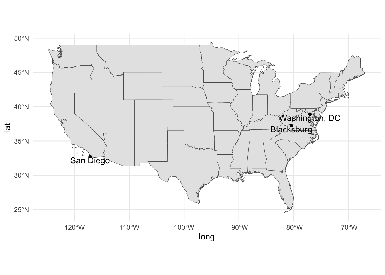
ggplot() +
  geom_sf(data = states) +
  geom_point(data = locations_geo, aes(x = long, y = lat)) +
  geom_text(data = locations_geo, aes(x = long, y = lat, label = name),
            nudge_y = -0.5) +
  theme_minimal()