8 Dates and times with lubridate

Published

April 12, 2023

Modified

January 8, 2024

These notes on lubridate are from the date and times chapter in R for Data Science.

library(tidyverse)
library(nycflights13)

8.1 Creating dates and date times

8.1.1 Getting the current date or time

# lubridate
today()
#> [1] "2024-01-08"
now()
#> [1] "2024-01-08 16:51:52 MST"

# Base
Sys.Date()
#> [1] "2024-01-08"
Sys.time()
#> [1] "2024-01-08 16:51:52 MST"

8.1.2 On import with readr

If your CSV contains an ISO8601 date or date-time, you do not need to do anything; readr will automatically recognize it.

You can also use col_date() with date components. Table Table 8.1 lists all the options.

Table 8.1: All date formats understood by readr

Type	Code	Meaning	Example
Year	`%Y`	4 digit year	2021
	`%y`	2 digit year	21
Month	`%m`	Number	2
	`%b`	Abbreviated name	Feb
	`%B`	Full name	February
Day	`%d`	Two digits	02
	`%e`	One or two digits	2
Time	`%H`	24-hour hour	13
	`%I`	12-hour hour	1
	`%p`	AM/PM	pm
	`%M`	Minutes	35
	`%S`	Seconds	45
	`%OS`	Seconds with decimal component	45.35
	`%Z`	Time zone name	America/Chicago
	`%z`	Offset from UTC	+0800
Other	`%.`	Skip one non-digit	:
	`%*`	Skip any number of non-digits

See the examples in the chapter on readr.

8.1.3 From strings

Using lubridate helper functions that use y for year, m for month, and d for day.

ymd("2023-04-12")
#> [1] "2023-04-12"
mdy("April 12th, 2023")
#> [1] "2023-04-12"
dmy("12-Apr-2023")
#> [1] "2023-04-12"

For a date time you add an underscore and h for hour, m for minute, and s for second.

ymd_hms("2023-04-12 09:32:24")
#> [1] "2023-04-12 09:32:24 UTC"
mdy_hm("04/12/2023 09:33")
#> [1] "2023-04-12 09:33:00 UTC"

8.1.4 From individual components

Use of make_date()

flights |> 
  select(year, month, day, hour, minute)
#> # A tibble: 336,776 × 5
#>     year month   day  hour minute
#>    <int> <int> <int> <dbl>  <dbl>
#>  1  2013     1     1     5     15
#>  2  2013     1     1     5     29
#>  3  2013     1     1     5     40
#>  4  2013     1     1     5     45
#>  5  2013     1     1     6      0
#>  6  2013     1     1     5     58
#>  7  2013     1     1     6      0
#>  8  2013     1     1     6      0
#>  9  2013     1     1     6      0
#> 10  2013     1     1     6      0
#> # ℹ 336,766 more rows

flights |> 
  select(year, month, day, hour, minute) |> 
  mutate(departure = make_datetime(year, month, day, hour, minute))
#> # A tibble: 336,776 × 6
#>     year month   day  hour minute departure          
#>    <int> <int> <int> <dbl>  <dbl> <dttm>             
#>  1  2013     1     1     5     15 2013-01-01 05:15:00
#>  2  2013     1     1     5     29 2013-01-01 05:29:00
#>  3  2013     1     1     5     40 2013-01-01 05:40:00
#>  4  2013     1     1     5     45 2013-01-01 05:45:00
#>  5  2013     1     1     6      0 2013-01-01 06:00:00
#>  6  2013     1     1     5     58 2013-01-01 05:58:00
#>  7  2013     1     1     6      0 2013-01-01 06:00:00
#>  8  2013     1     1     6      0 2013-01-01 06:00:00
#>  9  2013     1     1     6      0 2013-01-01 06:00:00
#> 10  2013     1     1     6      0 2013-01-01 06:00:00
#> # ℹ 336,766 more rows

flights lists most of the times in an odd format with hours and minutes combined into a single integer, so that 05:17 is 517. This can be split into hours and minutes with modulus arithmetic: h = x %/% 100 and m = x %% 100. We can create a function to create date times for departure and arrival times.

make_datetime_100 <- function(year, month, day, time) {
  make_datetime(year, month, day, time %/% 100, time %% 100)
}

flights_dt <- flights |> 
  filter(!is.na(dep_time), !is.na(arr_time)) |> 
  mutate(
    dep_time = make_datetime_100(year, month, day, dep_time),
    arr_time = make_datetime_100(year, month, day, arr_time),
    sched_dep_time = make_datetime_100(year, month, day, sched_dep_time),
    sched_arr_time = make_datetime_100(year, month, day, sched_arr_time)
  ) |> 
  select(origin, dest, ends_with("delay"), ends_with("time"))

flights_dt
#> # A tibble: 328,063 × 9
#>    origin dest  dep_delay arr_delay dep_time            sched_dep_time     
#>    <chr>  <chr>     <dbl>     <dbl> <dttm>              <dttm>             
#>  1 EWR    IAH           2        11 2013-01-01 05:17:00 2013-01-01 05:15:00
#>  2 LGA    IAH           4        20 2013-01-01 05:33:00 2013-01-01 05:29:00
#>  3 JFK    MIA           2        33 2013-01-01 05:42:00 2013-01-01 05:40:00
#>  4 JFK    BQN          -1       -18 2013-01-01 05:44:00 2013-01-01 05:45:00
#>  5 LGA    ATL          -6       -25 2013-01-01 05:54:00 2013-01-01 06:00:00
#>  6 EWR    ORD          -4        12 2013-01-01 05:54:00 2013-01-01 05:58:00
#>  7 EWR    FLL          -5        19 2013-01-01 05:55:00 2013-01-01 06:00:00
#>  8 LGA    IAD          -3       -14 2013-01-01 05:57:00 2013-01-01 06:00:00
#>  9 JFK    MCO          -3        -8 2013-01-01 05:57:00 2013-01-01 06:00:00
#> 10 LGA    ORD          -2         8 2013-01-01 05:58:00 2013-01-01 06:00:00
#> # ℹ 328,053 more rows
#> # ℹ 3 more variables: arr_time <dttm>, sched_arr_time <dttm>, air_time <dbl>

8.1.5 From other types

Use of as_datetime() and as_date() to switch between date-time and date.

as_datetime(today())
#> [1] "2024-01-08 UTC"
as_date(now())
#> [1] "2024-01-08"

To convert Unix Epoch to dates use as_datetime() if the offset is given in seconds and as_date() if it is given in days.

8.2 Date-time components

8.2.1 Getting components

Use of helper functions to get components of a date or date-time:

year()
month()
mday() day of the month
yday() day of the year
wday() day of the week
hour()
minute()
second()

datetime <- ymd_hms("2023-04-12 09:49:56")

year(datetime)
#> [1] 2023
month(datetime)
#> [1] 4
mday(datetime)
#> [1] 12

yday(datetime)
#> [1] 102
wday(datetime)
#> [1] 4

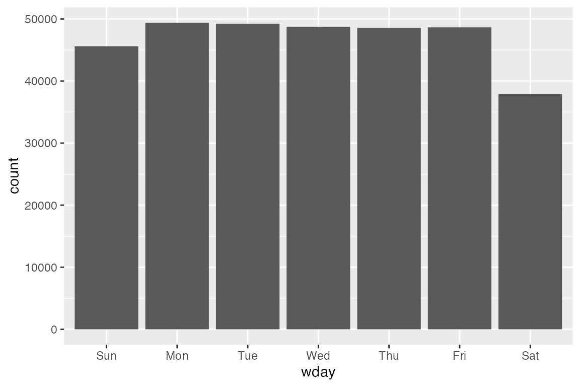
For month() and wday() you can set label = TRUE to return the abbreviated name of the month or day of the week. Set abbr = FALSE to return the full name.

month(datetime, label = TRUE)
#> [1] Apr
#> 12 Levels: Jan < Feb < Mar < Apr < May < Jun < Jul < Aug < Sep < ... < Dec
wday(datetime, label = TRUE, abbr = FALSE)
#> [1] Wednesday
#> 7 Levels: Sunday < Monday < Tuesday < Wednesday < Thursday < ... < Saturday

This can be used to plot flight departures by days of the week.

flights_dt |> 
  mutate(wday = wday(dep_time, label = TRUE)) |> 
  ggplot(aes(x = wday)) +
  geom_bar()

8.2.2 Rounding

Use of floor_date(), round_date(), and ceiling_date() to round dates to a given unit.

Valid units for rounding: second, minute, hour, day, week, month, bimonth, quarter, season, halfyear and year, or a Period object.

With rounding you can plot the number of flights per week:

flights_dt |> 
  count(week = floor_date(dep_time, "week")) |> 
  ggplot(aes(x = week, y = n)) +
  geom_line() + 
  geom_point()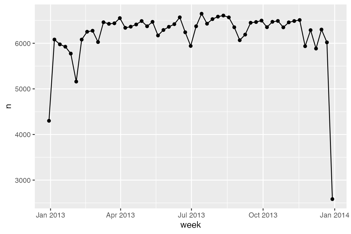

8.2.3 Modifying components

Modifying individual components:

datetime
#> [1] "2023-04-12 09:49:56 UTC"

year(datetime) <- 2030
month(datetime) <- 01
hour(datetime) <- hour(datetime) + 1
datetime
#> [1] "2030-01-12 10:49:56 UTC"

Or you can create a new date-time with update():

update(datetime, year = 2023, month = 04, hour = 10, minute = 23)
#> [1] "2023-04-12 10:23:56 UTC"

8.3 Time spans

Arithmetic with math leads to the use of three classes that represent time spans.

Durations: represent an exact number of seconds.
Periods: represent human units like weeks and months.
Intervals: represent a starting and ending point.

8.3.1 Durations

Arithmetic with dates in R creates a difftime object, which records a time span of seconds, minutes, hours, days, or weeks. This can lead to ambiguity, so lubridate provides Duration, which always records time spans in seconds.

# Base difftime
age <- today() - ymd("1983-03-28")
age
#> Time difference of 14896 days

# duration
as.duration(age)
#> [1] "1287014400s (~40.78 years)"

Durations have a variety of constructors.

dminutes(10)
#> [1] "600s (~10 minutes)"
ddays(0:5)
#> [1] "0s"                "86400s (~1 days)"  "172800s (~2 days)"
#> [4] "259200s (~3 days)" "345600s (~4 days)" "432000s (~5 days)"

Note that because durations are seconds there can be some ambiguity with larger units. Months cannot be calculated and years are set to an average of 365.25 days.

8.3.2 Periods

To deal with the ambiguities of Duration lubridate implements the [Period type](https://lubridate.tidyverse.org/reference/index.html#periods. Period constructors:

hours(c(12, 24))
#> [1] "12H 0M 0S" "24H 0M 0S"
days(7)
#> [1] "7d 0H 0M 0S"
10 * (months(6) + days(1))
#> [1] "60m 10d 0H 0M 0S"

Compared to durations, periods are more likely to do what you expect:

# A leap year
ymd("2024-01-01") + dyears(1)
#> [1] "2024-12-31 06:00:00 UTC"
ymd("2024-01-01") + years(1)
#> [1] "2025-01-01"

# Daylight Savings Time
one_am <- ymd_hms("2026-03-08 01:00:00", tz = "America/New_York")
one_am + ddays(1)
#> [1] "2026-03-09 02:00:00 EDT"
one_am + days(1)
#> [1] "2026-03-09 01:00:00 EDT"

Can use periods to fix a problem in the flights_dt data. Overnight flights appear to arrive before they depart because the date was calculated on the departure date. This can be fixed by adding days(1) to the arrival times of overnight flights using the fact that TRUE == 1.

# Number of overnight flights
flights_dt |> 
  filter(arr_time < dep_time) |> 
  nrow()
#> [1] 10633

flights_dt <- flights_dt |> 
  mutate(
    overnight = arr_time < dep_time,
    arr_time = arr_time + days(overnight),
    sched_arr_time = sched_arr_time + days(overnight)
  )

# Now fixed
flights_dt |> 
  filter(arr_time < dep_time) |> 
  nrow()
#> [1] 0

8.3.3 Intervals

For accurate measurement between specific dates and date-times you can use intervals.

Create an intervalby writing start %--% end:

# Periods use estimates of length
years(1) / days(1)
#> [1] 365.25

# Intervals are specific
y2023 <- ymd("2023-01-01") %--% ymd("2024-01-01")
y2024 <- ymd("2024-01-01") %--% ymd("2025-01-01")

y2023 / days(1)
#> [1] 365
y2024 / days(1)
#> [1] 366

8.4 Time zones

R uses the international standard IANA time zones. These use a consistent naming scheme {area}/{location}, typically in the form {continent}/{city} or {ocean}/{city}. These two pieces of information are useful for recording the history of how time zones might change in different places. You can see this in the IANA database of time zones.

# Locale time zone
Sys.timezone()
#> [1] "America/Mazatlan"

# List of time zones
head(OlsonNames())
#> [1] "Africa/Abidjan"     "Africa/Accra"       "Africa/Addis_Ababa"
#> [4] "Africa/Algiers"     "Africa/Asmara"      "Africa/Asmera"

Time zones only affect printing, not the recording of the actual time.

x <- ymd_hms("2023-04-12 11:23:00", tz = "America/New_York")
y <- ymd_hms("2023-04-12 17:23:00", tz = "Europe/Copenhagen")

x - y
#> Time difference of 0 secs

lubridate uses UTC (Coordinated Universal Time) as a default. UTC is roughly equivalent to GMT (Greenwich Mean Time), but it does not have DST, which makes a convenient representation for computation.

You can change time zones by either changing how it is displayed or altering the underlying instant in time. c() drops time zones and displays them in your locale.

# Convert to local time zone
z <- c(x, y)

# Change time zone representation
za <- with_tz(z, tzone = "Australia/Lord_Howe")
za
#> [1] "2023-04-13 01:53:00 +1030" "2023-04-13 01:53:00 +1030"

z - za
#> Time differences in secs
#> [1] 0 0

# Change instant and time zone
zb <- force_tz(z, tzone = "Australia/Lord_Howe")
zb
#> [1] "2023-04-12 11:23:00 +1030" "2023-04-12 11:23:00 +1030"

z - zb
#> Time differences in hours
#> [1] 14.5 14.5