All in One View
Content from Before we start
Last updated on 2026-04-28 | Edit this page
Overview
Questions
- Why should you use R and RStudio?
- How do you get started working in R and RStudio?
Objectives
- Understand the difference between R and RStudio
- Describe the purpose of the different RStudio panes
- Organize files and directories into R Projects
- Use the RStudio help interface to get help with R functions
- Be able to format questions to get help in the broader R community
What is R? What is RStudio?
The term “R” is used to refer to both the programming
language and the software that interprets the scripts written using
it.
RStudio is a popular way to write R scripts and interact with the R software. To function correctly, RStudio needs R and therefore both need to be installed on your computer.
Why learn R?
R does not involve lots of pointing and clicking, and that’s a good thing
In R, the results of your analysis rely on a series of written commands, and not on remembering a succession of pointing and clicking. That is a good thing! So, if you want to redo your analysis because you collected more data, you don’t have to remember which button you clicked in which order to obtain your results. With a stored series of commands in an R script, you can repeat running them and R will process the new dataset exactly the same way as before.
Working with scripts makes the steps you used in your analysis clear, and the code you write can be inspected by someone else who can give you feedback and spot mistakes.
Working with scripts forces you to have a deeper understanding of what you are doing, and facilitates your learning and comprehension of the methods you use.
R code is great for reproducibility
Reproducibility is when someone else, including your future self, can obtain the same results from the same dataset when using the same analysis.
R integrates with other tools to generate manuscripts from your code. If you collect more data, or fix a mistake in your dataset, the figures and the statistical tests in your manuscript are updated automatically.
R is widely used in academia and in industries such as pharma and biotech. These organisations expect analyses to be reproducible, so knowing R will give you an edge with these requirements.
R is interdisciplinary and extensible
With 10,000+ packages that can be installed to extend its capabilities, R provides a framework that allows you to combine statistical approaches from many scientific disciplines to best suit the analytical framework you need to analyze your data. For instance, R has packages for image analysis, GIS, time series, population genetics, and a lot more.
R works on data of all shapes and sizes
The skills you learn with R scale easily with the size of your dataset. Whether your dataset has hundreds or millions of lines, it won’t make much difference to you.
R is designed for data analysis. It comes with special data structures and data types that make handling of missing data and statistical factors convenient.
R can connect to spreadsheets, databases, and many other data formats, on your computer or on the web.
R produces high-quality graphics
The plotting functionalities in R are endless, and allow you to adjust any aspect of your graph to visualize your data more effectively.
R has a large and welcoming community
Thousands of people use R daily. Many of them are willing to help you
through mailing lists and websites such as Stack Overflow, RStudio community, and Slack
channels such as
the R for Data Science online community (https://www.rfordatasci.com/).
In addition, there are numerous online and in person meetups organised
globally through organisations such as R Ladies Global (https://rladies.org/).
Knowing your way around RStudio
Let’s start by learning about RStudio, which is an Integrated Development Environment (IDE) for working with R.
The RStudio IDE open-source product is free under the Affero General Public License (AGPL) v3. The RStudio IDE is also available with a commercial license and priority email support from RStudio, PBC.
We will use RStudio IDE to write code, navigate the files on our computer, inspect the variables we are going to create, and visualize the plots we will generate. RStudio can also be used for other things (e.g., version control, developing packages, writing Shiny apps) that we will not cover during the workshop.
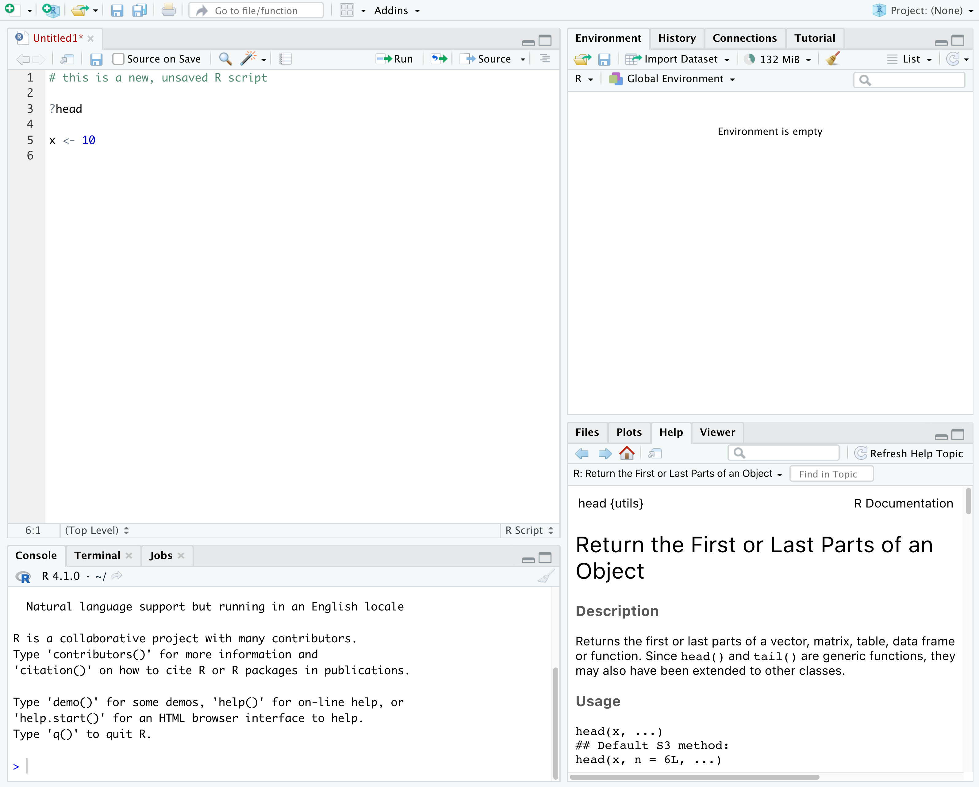
RStudio is divided into 4 “panes”:
- The Source for your scripts and documents (top-left, in the default layout)
- Your Environment/History (top-right) which shows all the objects in your working space (Environment) and your command history (History)
- Your Files/Plots/Packages/Help/Viewer (bottom-right)
- The R Console (bottom-left)
The placement of these panes and their content can be customized (see
menu, Tools --> Global Options --> Pane Layout). For
ease of use, settings such as background color, font color, font size,
and zoom level can also be adjusted in this menu
(Global Options --> Appearance).
One of the advantages of using RStudio is that all the information you need to write code is available in a single window. Additionally, with many shortcuts, autocompletion, and highlighting for the major file types you use while developing in R, RStudio will make typing easier and less error-prone.
Getting set up
It is good practice to keep a set of related data, analyses, and text self-contained in a single folder, called the working directory. All of the scripts within this folder can then use relative paths to files that indicate where inside the project a file is located (as opposed to absolute paths, which point to where a file is on a specific computer). Working this way allows you to move your project around on your computer and share it with others without worrying about whether or not the underlying scripts will still work.
RStudio provides a helpful set of tools to do this through its “Projects” interface, which not only creates a working directory for you, but also remembers its location (allowing you to quickly navigate to it) and optionally preserves custom settings and (re-)open files to assist resume work after a break. Go through the steps for creating an “R Project” for this tutorial below.
- Start RStudio.
- Under the
Filemenu, click onNew Project. ChooseNew Directory, thenNew Project. - Enter a name for this new folder (or “directory”), and choose a
convenient location for it. This will be your working
directory for the rest of the day (e.g.,
~/r-ecology). - Click on
Create Project.
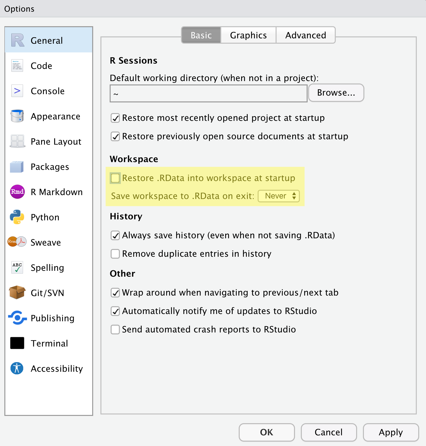
A workspace is your current working environment in R which includes
any user-defined object. By default, all of these objects will be saved,
and automatically loaded, when you reopen your project. Saving a
workspace to .RData can be cumbersome, especially if you
are working with larger datasets, and it can lead to hard to debug
errors by having objects in memory you forgot you had. Therefore, it is
often a good idea to turn this off. To do so, go to
Tools --> Global Options and uncheck
Restore .RData into workspace at startup and select the
‘Never’ option for
Save workspace to .RData' on exit.
Organizing your working directory
Using a consistent folder structure across your projects will help keep things organized, and will help you to find/file things in the future. This can be especially helpful when you have multiple projects. In general, you may create directories (folders) for scripts, data, plots, and documents.
-
data_raw/&data/- Use these folders to store raw data and intermediate datasets you may create for the need of a particular analysis. For the sake of transparency and provenance, you should always keep a copy of your raw data accessible and do as much of your data cleanup and preprocessing programmatically (i.e., with scripts, rather than manually) as possible.
- Separating raw data from processed data is also a good idea. For
example, you could have files
data_raw/tree_survey.plot1.txtand...plot2.txtkept separate from adata/tree.survey.csvfile generated by thescripts/01.preprocess.tree_survey.Rscript.
-
scripts/This would be the location to keep your R scripts for different analyses or plotting, and potentially a separate folder for functions that you might create. -
fig/This is a location for the plots that you make with your scripts. -
documents/This would be a place to keep outlines, drafts, and other text. - Additional (sub)directories depending on your project needs.
For this workshop, we will need a data_raw/ folder to
store our raw data, and we will use data/ for when we learn
how to export data as CSV files, and a fig/ folder for the
figures that we will save.
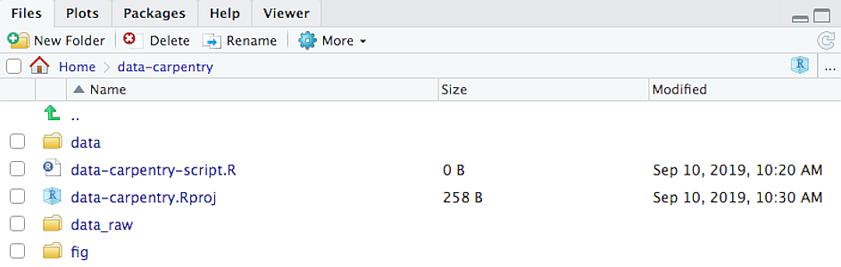
- Under the
Filestab on the right of the screen, click onNew Folderand create a folder nameddata_rawwithin your newly created working directory (e.g.,~/data-carpentry/). (Alternatively, typedir.create("data_raw")at your R console.) Repeat these operations to create adataand afigfolder.
We are going to keep the script in the root of our working directory because we are only going to use one file. Later, when you start create more complex projects, it might make sense to organize scripts in sub-directories.
Your working directory should now look like this:
Interacting with R
The basis of programming is that we write down instructions for the computer to follow, and then we tell the computer to follow those instructions. We write these instructions in the form of code, which is a common language that is understood by the computer and humans (after some practice). We call these instructions commands, and we tell the computer to follow the instructions by running (also called executing) the commands.
Console vs. script
You can run commands directly in the R console, or you can write them into an R script. It may help to think of working in the console vs. working in a script as something like cooking. The console is like making up a new recipe, but not writing anything down. You can carry out a series of steps and produce a nice, tasty dish at the end. However, because you didn’t write anythingdown, it’s harder to figure out exactly what you did, and in what order.
Writing a script is like taking nice notes while cooking- you can tweak and edit the recipe all you want, you can come back in 6 months and try it again, and you don’t have to try to remember what went well and what didn’t. It’s actually even easier than cooking, since you can hit one button and the computer “cooks” the whole recipe for you!
An additional benefit of scripts is that you can leave
comments for yourself or others to read. Lines that
start with # are considered comments and will not be
interpreted as R code.
Console
- The R console is where code is run/executed
- The prompt, which is the
>symbol, is where you can type commands - By pressing Enter, R will execute those commands and print the result.
- You can work here, and your history is saved in the History pane, but you can’t access it in the future
Script
- A script is a record of commands to send to R, preserved in a plain
text file with a
.Rextension - You can make a new R script by clicking
File → New File → R Script, clicking the green+button in the top left corner of RStudio, or pressing Shift+Cmd+N (Mac) or Shift+Ctrl+N (Windows). It will be unsaved, and called “Untitled1” - If you type out lines of R code in a script, you can send them to
the R console to be evaluated
- Cmd+Enter (Mac) or Ctrl+Enter (Windows) will run the line of code that your cursor is on
- If you highlight multiple lines of code, you can run all of them by pressing Cmd+Enter (Mac) or Ctrl+Enter (Windows)
- By preserving commands in a script, you can edit and rerun them quickly, save them for later, and share them with others
- You can leave comments for yourself by starting a line with a
#or placing#after a line of code.
Example
Let’s try running some code in the console and in a script. First,
click down in the Console pane, and type out 1+1. Hit
Enter to run the code. You should see your code echoed, and
then the value of 2 returned.
Now click into your blank script, and type out 1+1. With
your cursor on that line, hit Cmd+Enter (Mac) or
Ctrl+Enter (Windows) to run the code. You will see that your
code was sent from the script to the console, where it returned a value
of 2, just like when you ran your code directly in the
console.
Now save and name the script that we will be working on for the rest
of the workshop. You might name it intro.R. Try to choose
simple, memorable names for your scripts and avoid using spaces.
Seeking help
Searching function documentation with ? and
??
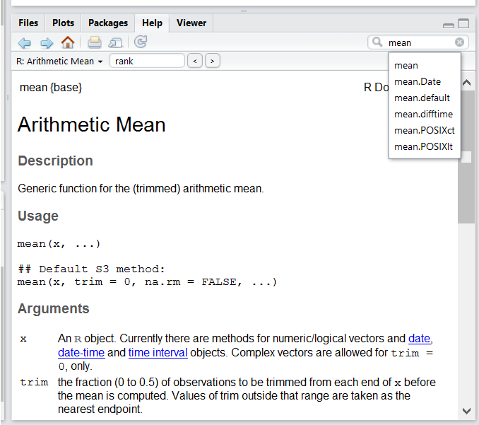
If you need help with a specific function, let’s say
mean(), you can type ?mean or press
F1 while your cursor is on the function name. If you are
looking for a function to do a particular task, but don’t know the
function name, you can use the double question mark ??, for
example ??kruskall. Both commands will open matching help
files in RStudio’s help panel in the lower right corner. You can also
use the help panel to search help directly, as seen in the
screenshot.
Automatic code completion
When you write code in RStudio, you can use its automatic code completion to remind yourself of a function’s name or arguments. Start typing the function name and pay attention to the suggestions that pop up. Use the up and down arrow to select a suggested code completion and Tab to apply it. You can also use code completion to complete function’s argument names, object, names and file names. It even works if you don’t get the spelling 100% correct.
Package vignettes and cheat sheets
In addition to the documentation for individual functions, many
packages have vignettes – instructions for how to use the
package to do certain tasks. Vignettes are great for learning by
example. Vignettes are accessible via the package help and by using the
function browseVignettes().
There is also a Help menu at the top of the RStudio window, that has cheat sheets for popular packages, RStudio keyboard shortcuts, and more.
Finding more functions and packages
RStudio’s help only searches the packages that you have installed on your machine, but there are many more available on CRAN and GitHub. To search across all available R packages, you can use the website rdocumentation.org. Often, a generic Google or internet search “R <task>” will send you to the appropriate package documentation or a forum where someone else has already asked your question. Many packages also have websites with additional help, tutorials, news and more (for example tidyverse.org).
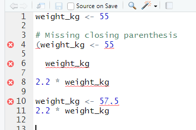
Dealing with error messages
Don’t get discouraged if your code doesn’t run immediately! Error messages are common when programming, and fixing errors is part of any programmer’s daily work. Often, the problem is a small typo in a variable name or a missing parenthesis. Watch for the red x’s next to your code in RStudio. These may provide helpful hints about the source of the problem.
If you can’t fix an error yourself, start by googling it. Some error messages are too generic to diagnose a problem (e.g. “subscript out of bounds”). In that case it might help to include the name of the function or package you’re using in your query.
Asking for help
If your Google search is unsuccessful, you may want to ask other R users for help. There are different places where you can ask for help. During this workshop, don’t hesitate to talk to your neighbor, compare your answers, and ask for help. You might also be interested in organizing regular meetings following the workshop to keep learning from each other. If you have a friend or colleague with more experience than you, they might also be able and willing to help you.
Learning to search for help is probably the most useful skill for any
R user. The key skill is figuring out what you should actually search
for. It’s often a good idea to start your search with R or
R programming. If you have the name of a package you want
to use, start with R package_name.
Many of the answers you find will be from a website called Stack Overflow, where people ask programming questions and others provide answers.
Generative AI Help
In addition to the resources we’ve already mentioned for getting help with R, it’s becoming increasingly common to turn to generative AI chatbots such as ChatGPT to get help while coding. You will probably receive some useful guidance by presenting your error message to the chatbot and asking it what went wrong.
However, the way this help is provided by the chatbot is different. Answers on Stack Overflow have (probably) been given by a human as a direct response to the question asked. But generative AI chatbots, which are based on an advanced statistical model, respond by generating the most likely sequence of text that would follow the prompt they are given.
While responses from generative AI tools can often be helpful, they are not always reliable. These tools sometimes generate plausible but incorrect or misleading information, so (just as with an answer found on the internet) it is essential to verify their accuracy. You need the knowledge and skills to be able to understand these responses, to judge whether or not they are accurate, and to fix any errors in the code it offers you.
In addition to asking for help, programmers can use generative AI tools to generate code from scratch; extend, improve and reorganise existing code; translate code between programming languages; figure out what terms to use in a search of the internet; and more. However, there are drawbacks that you should be aware of.
The models used by these tools have been “trained” on very large volumes of data, much of it taken from the internet, and the responses they produce reflect that training data, and may recapitulate its inaccuracies or biases. The environmental costs (energy and water use) of LLMs are a lot higher than other technologies, both during development (known as training) and when an individual user uses one (also called inference). For more information see the AI Environmental Impact Primer developed by researchers at HuggingFace, an AI hosting platform. Concerns also exist about the way the data for this training was obtained, with questions raised about whether the people developing the LLMs had permission to use it. Other ethical concerns have also been raised, such as reports that workers were exploited during the training process.
We recommend that you avoid getting help from generative AI during the workshop for several reasons:
- For most problems you will encounter at this stage, help and answers can be found among the first results returned by searching the internet.
- The foundational knowledge and skills you will learn in this lesson by writing and fixing your own programs are essential to be able to evaluate the correctness and safety of any code you receive from online help or a generative AI chatbot. If you choose to use these tools in the future, the expertise you gain from learning and practising these fundamentals on your own will help you use them more effectively.
- As you start out with programming, the mistakes you make will be the kinds that have also been made – and overcome! – by everybody else who learned to program before you. Since these mistakes and the questions you are likely to have at this stage are common, they are also better represented than other, more specialised problems and tasks in the data that was used to train generative AI tools. This means that a generative AI chatbot is more likely to produce accurate responses to questions that novices ask, which could give you a false impression of how reliable they will be when you are ready to do things that are more advanced.
How to learn more after the workshop?
The material we cover during this workshop will give you a taste of how you can use R to analyze data for your own research. However, to do advanced operations such as cleaning your dataset, using statistical methods, or creating beautiful graphics you will need to learn more.
The best way to become proficient and efficient at R, as with any other tool, is to use it to address your actual research questions. As a beginner, it can feel daunting to have to write a script from scratch, and given that many people make their code available online, modifying existing code to suit your purpose might get first hands-on experience using R for your own work and help you become comfortable eventually creating your own scripts.
More resources
More about R
- Hadley Wickham, Mine Çetinkaya-Rundel, and Garrett Grolemund, R for Data Science, Second edition (2023)
- R-bloggers
- Tidyverse - Website for the tidyverse packages, full of the documentation and vignettes.
- Posit Community - Good place to look for answers to questions about R.
- Tidy Tuesday - Weekly social data project. New data every week.
- R Graph Gallery
How to ask good programming questions?
- The rOpenSci community call “How to ask questions so they get answered”, (rOpenSci site and video recording) includes a presentation of the reprex package and of its philosophy.
- blog.Revolutionanalytics.com and this blog post by Jon Skeet have comprehensive advice on how to ask programming questions.
Content from Introduction to R
Last updated on 2026-04-28 | Edit this page
Overview
Questions
- How do you create variables in R?
- What are the main types of vectors in R?
Objectives
- Define the following terms as they relate to R: object, assign, call, function, arguments, options.
- Create objects and assign values to them in R.
- Learn how to name objects.
- Save a script file for later use.
- Use comments to inform script.
- Solve simple arithmetic operations in R.
- Call functions and use arguments to change their default options.
- Inspect the content of vectors and manipulate their content.
- Subset and extract values from vectors.
- Analyze vectors with missing data.
Note: This lesson is a shortened and modified version of the Data Carpentry Ecology R Lesson. Please refer to the original for additional functions and examples, as well as regular updates.
Creating objects in R
You can get output from R simply by typing math in the console:
R
3 + 5
12 / 7
However, to do useful and interesting things, we need to assign
values to objects. To create an object, we need to
give it a name followed by the assignment operator <-,
and the value we want to give it:
R
weight_kg <- 55
<- is the assignment operator. It assigns values on
the right to objects on the left. So, after executing
x <- 3, the value of x is 3.
For historical reasons, you can also use = for assignments,
but not in every context. Because of the slight
differences
in syntax, it is good practice to always use <- for
assignments.
Objects can be given almost any name such as x,
current_temperature, or subject_id. Here are
some further guidelines on naming objects:
- You want your object names to be explicit and not too long.
- They cannot start with a number (
2xis not valid, butx2is). - R is case sensitive, so for example,
weight_kgis different fromWeight_kg. - Don’t use function names of fundamental functions in R (e.g.,
if,else,for,c,T,mean,data,df,weights, etc.). If in doubt, check the help to see if the name is already in use. - Avoid dots (
.) within names. - Be consistent in the styling of your code, such as where you put spaces, how you name objects, etc. Styles can include “lower_snake”, “UPPER_SNAKE”, “lowerCamelCase”, “UpperCamelCase”, etc.
Objects vs. variables
What are known as objects in R are known as
variables in many other programming languages. Depending on
the context, object and variable can have
drastically different meanings. However, in this lesson, the two words
are used synonymously. For more information see: https://cran.r-project.org/doc/manuals/r-release/R-lang.html#Objects
When assigning a value to an object, R does not print anything. You can force R to print the value by typing the object name:
R
weight_kg <- 55    # doesn't print anything
weight_kg          # but typing the name of the object does (once it's created)
Now that R has weight_kg in memory, we can do arithmetic
with it. For instance, we may want to convert this weight into pounds
(weight in pounds is 2.2 times the weight in kg):
R
2.2 * weight_kg
We can also change an object’s value by assigning it a new one:
R
weight_kg <- 57.5
2.2 * weight_kg
Assigning a value to one object does not change the values of other
objects. For example, let’s store the animal’s weight in pounds in a new
object, weight_lb:
R
weight_lb <- 2.2 * weight_kg
and then change weight_kg to 100.
R
weight_kg <- 100
What do you think is the current content of the object
weight_lb? 126.5 or 220?
Functions and their arguments
Functions are “canned scripts” that automate more complicated sets of
commands including operations assignments, etc. Many functions are
predefined, or can be made available by importing R packages
(more on that later). A function usually takes one or more inputs called
arguments. Functions often (but not always) return a
value. A typical example would be the function
round(). The input (the argument) must be a number, and the
return value (in fact, the output) is the input rounded to the nearest
whole number. Executing a function (‘running it’) is called
calling the function. An example of a function call is:
R
round(3.14159)
OUTPUT
#> [1] 3Here, we’ve called round() with just one argument,
3.14159, and it has returned the value 3.
That’s because the default is to round to the nearest whole number.
The return ‘value’ of a function need not be numerical, and it also does not need to be a single item: it can be a set of things, or even a dataset. We’ll see that when we read data files into R.
Arguments can be anything, not only numbers or filenames, but also other objects. Exactly what each argument means differs per function, and must be looked up in the documentation (see below). Some functions take arguments which may either be specified by the user, or, if left out, take on a default value: these are called options. Options are typically used to alter the way the function operates, such as whether it ignores ‘bad values’, or what symbol to use in a plot. However, if you want something specific, you can specify a value of your choice which will be used instead of the default.
If we want more digits we can see how to do that by getting
information about the round function. We can use
args(round) to find what arguments it takes, or look at the
help for this function using ?round.
R
args(round)
OUTPUT
#> function (x, digits = 0, ...)
#> NULL
R
?round
We see that if we want a different number of digits, we can type
digits = 2 or however many we want.
R
round(3.14159, digits = 2)
OUTPUT
#> [1] 3.14If you provide the arguments in the exact same order as they are defined you don’t have to name them:
R
round(3.14159, 2)
OUTPUT
#> [1] 3.14And if you do name the arguments, you can switch their order:
R
round(digits = 2, x = 3.14159)
OUTPUT
#> [1] 3.14It’s good practice to put the non-optional arguments (like the number you’re rounding) first in your function call, and to then specify the names of all optional arguments. If you don’t, someone reading your code might have to look up the definition of a function with unfamiliar arguments to understand what you’re doing.
Vectors and data types
A vector is the most common and basic data type in R, and is pretty
much the workhorse of R. A vector is composed by a series of values,
which can be either numbers or characters. We can assign a series of
values to a vector using the c() function. For example we
can create a vector of animal weights and assign it to a new object
weight_g:
R
weight_g <- c(50, 60, 65, 82)
weight_g
A vector can also contain characters:
R
animals <- c("mouse", "rat", "dog")
animals
The quotes around “mouse”, “rat”, etc. are essential here. Without
the quotes R will assume objects have been created called
mouse, rat and dog. As these
objects don’t exist in R’s memory, there will be an error message.
There are many functions that allow you to inspect the content of a
vector. length() tells you how many elements are in a
particular vector:
R
length(weight_g)
length(animals) #notice this doesn't return the number of characters
An important feature of a vector, is that all of the elements are the
same type of data. The function class() indicates what kind
of object you are working with:
R
class(weight_g)
class(animals)
The function str() provides an overview of the structure
of an object and its elements. It is a useful function when working with
large and complex objects:
R
str(weight_g)
str(animals)
You can use the c() function to add other elements to
your vector:
R
weight_g <- c(weight_g, 90) # add to the end of the vector
weight_g <- c(30, weight_g) # add to the beginning of the vector
weight_g
In the first line, we take the original vector weight_g,
add the value 90 to the end of it, and save the result back
into weight_g. Then we add the value 30 to the
beginning, again saving the result back into weight_g.
We can do this over and over again to grow a vector, or assemble a dataset. As we program, this may be useful to add results that we are collecting or calculating.
An atomic vector is the simplest R data
type and is a linear vector of a single type. Above, we saw 2
of the 6 main atomic vector types that R uses:
"character" and "numeric" (or
"double"). These are the basic building blocks that all R
objects are built from. The other 4 atomic vector types
are:
-
"logical"forTRUEandFALSE(the boolean data type) -
"integer"for integer numbers (e.g.,2L, theLindicates to R that it’s an integer) -
"complex"to represent complex numbers with real and imaginary parts (e.g.,1 + 4i) and that’s all we’re going to say about them -
"raw"for bitstreams that we won’t discuss further
You can check the type of your vector using the typeof()
function and inputting your vector as the argument.
Vectors are one of the many data structures that R
uses. Other important types you may encounter are lists
(list), matrices (matrix), data frames
(data.frame), factors (factor) and arrays
(array).
Challenge
- We’ve seen that atomic vectors can be of type character, numeric (or double), integer, and logical. But what happens if we try to mix these types in a single vector?
R implicitly converts them to all be the same type
Challenge (continued)
-
What will happen in each of these examples? (hint: use
class()to check the data type of your objects):R
num_char <- c(1, 2, 3, "a")
num_logical <- c(1, 2, 3, TRUE)
char_logical <- c("a", "b", "c", TRUE)
tricky <- c(1, 2, 3, "4")
Why do you think it happens?
Vectors can be of only one data type. R tries to convert (coerce) the content of this vector to find a “common denominator” that doesn’t lose any information.
Challenge (continued)
-
How many values in
combined_logicalare"TRUE"(as a character) in the following example (reusing the 2..._logicals from above):R
combined_logical <- c(num_logical, char_logical)
Only one. There is no memory of past data types, and the coercion
happens the first time the vector is evaluated. Therefore, the
TRUE in num_logical gets converted into a
1 before it gets converted into "1" in
combined_logical.
Challenge (continued)
- You’ve probably noticed that objects of different types get converted into a single, shared type within a vector. In R, we call converting objects from one class into another class coercion. These conversions happen according to a hierarchy, whereby some types get preferentially coerced into other types. Can you draw a diagram that represents the hierarchy of how these data types are coerced?
logical → numeric → character ← logical
Subsetting vectors
If we want to extract one or several values from a vector, we must provide one or several indices in square brackets. For instance:
R
animals <- c("mouse", "rat", "dog", "cat")
animals[2]
OUTPUT
#> [1] "rat"R
animals[c(3, 2)]
OUTPUT
#> [1] "dog" "rat"Program in other languages?
R indices start at 1. Some other languages (like C++, Java, Perl, and Python) count from 0 because that’s simpler for computers to do.
Conditional subsetting
Another common way of subsetting is by selecting only values where a
condition is TRUE. To do so, we use the []
notation with a logical test:
R
## we can use this to select only the values above 50
weight_g[weight_g > 50]
OUTPUT
#> [1] 60 65 82 90You can combine multiple tests using & (both
conditions are true, AND) or | (at least one of the
conditions is true, OR):
R
weight_g[weight_g > 30 & weight_g < 50]
OUTPUT
#> numeric(0)R
weight_g[weight_g <= 30 | weight_g == 55]
OUTPUT
#> [1] 30R
weight_g[weight_g >= 30 & weight_g == 21]
OUTPUT
#> numeric(0)Here, > for “greater than”, < stands
for “less than”, <= for “less than or equal to”, and
== for “equal to”. The double equal sign == is
a test for numerical equality between the left and right hand sides, and
should not be confused with the single = sign, which
performs variable assignment (similar to <-).
A common task is to search for certain strings in a vector. One could
use the “or” operator | to test for equality to multiple
values, but this can quickly become tedious. The function
%in% allows you to test if any of the elements of a search
vector are found:
R
animals <- c("mouse", "rat", "dog", "cat", "cat")

# use the logical vector created by %in% to return elements from animals
# that are found in the character vector
animals[animals %in% c("rat", "cat", "dog")]
OUTPUT
#> [1] "rat" "dog" "cat" "cat"Missing data
As R was designed to analyze datasets, it includes the concept of
missing data (which is uncommon in other programming languages). Missing
data are represented in vectors as NA.
When doing operations on numbers, most functions will return
NA if the data you are working with include missing values.
This feature makes it harder to overlook the cases where you are dealing
with missing data. You can add the argument na.rm = TRUE to
calculate the result as if the missing values were removed
(rm stands for ReMoved) first.
R
heights <- c(2, 4, 4, NA, 6)
mean(heights)
max(heights)
mean(heights, na.rm = TRUE)
max(heights, na.rm = TRUE)
If your data include missing values, you may want to become familiar
with the functions is.na(), na.omit(), and
complete.cases(). See below for examples.
R
## Extract those elements which are not missing values.
heights[!is.na(heights)]

## Returns the object with incomplete cases removed.
#The returned object is an atomic vector of type `"numeric"` (or #`"double"`).
na.omit(heights)

## Extract those elements which are complete cases.
#The returned object is an atomic vector of type `"numeric"` (or #`"double"`).
heights[complete.cases(heights)]
Recall that you can use the typeof() function to find
the type of your atomic vector.
Challenge
- Using this vector of heights in inches, create a new vector,
heights_no_na, with the NAs removed.
R
heights <- c(63, 69, 60, 65, NA, 68, 61, 70, 61, 59, 64, 69, 63, 63, NA, 72, 65, 64, 70, 63, 65)
Use the function
median()to calculate the median of theheightsvector.Use R to figure out how many people in the set are taller than 67 inches.
R
heights <- c(63, 69, 60, 65, NA, 68, 61, 70, 61, 59, 64, 69, 63, 63, NA, 72, 65, 64, 70, 63, 65)

# 1.
heights_no_na <- heights[!is.na(heights)]
# or
heights_no_na <- na.omit(heights)
# or
heights_no_na <- heights[complete.cases(heights)]

# 2.
median(heights, na.rm = TRUE)

# 3.
heights_above_67 <- heights_no_na[heights_no_na > 67]
length(heights_above_67)
Now that we have learned how to write scripts, and the basics of R’s data structures, we are ready to start working with a real dataset and learn about data frames.
Content from Working with data in the tidyverse
Last updated on 2026-04-28 | Edit this page
Overview
Questions
- How do you work with tabular data in R
- Why use the tidyverse to wrangle data?
Objectives
- Load external data from a .csv file into a data frame.
- Install and load packages.
- Describe what a data frame is.
- Summarize the contents of a data frame.
- Wrangle data with dplyr.
- Export a data frame to a .csv file.
Loading the survey data
We are investigating the animal species diversity and weights found within plots at our study site. The dataset is stored as a comma separated value (CSV) file. Each row holds information for a single animal, and the columns represent:
| Column | Description |
|---|---|
| record_id | Unique id for the observation |
| month | month of observation |
| day | day of observation |
| year | year of observation |
| plot_id | ID of a particular experimental plot of land |
| species_id | 2-letter code |
| sex | sex of animal (“M”, “F”) |
| hindfoot_length | length of the hindfoot in mm |
| weight | weight of the animal in grams |
| genus | genus of animal |
| species | species of animal |
| taxon | e.g. Rodent, Reptile, Bird, Rabbit |
| plot_type | type of plot |
Downloading the data
We created the folder that will store the downloaded data
(data_raw) in the chapter “Before
we start”. If you skipped that part, it may be a good idea to have a
look now, to make sure your working directory is set up properly.
We are going to use the R function download.file() to
download the CSV file that contains the survey data from Figshare, and
we will use read_csv() to load the content of the CSV file
into R.
Inside the download.file command, the first entry is a
character string with the source URL (“https://ndownloader.figshare.com/files/2292169”). This
source URL downloads a CSV file from figshare. The text after the comma
(“data_raw/portal_data_joined.csv”) is the destination of the file on
your local machine. You’ll need to have a folder on your machine called
“data_raw” where you’ll download the file. So this command downloads a
file from Figshare, names it “portal_data_joined.csv” and adds it to a
preexisting folder named “data_raw”.
R
download.file(url = "https://ndownloader.figshare.com/files/2292169",
              destfile = "data_raw/portal_data_joined.csv")
Reading the data into R
The file has now been downloaded to the destination you specified,
but R has not yet loaded the data from the file into memory. To do this,
we can use the read_csv() function from the
`readr`` package.
Packages in R are basically sets of additional functions that let you
do more stuff. The functions we’ve been using so far, like
round(), sqrt(), or c() come
built into R. Packages give you access to additional functions beyond
base R. A similar function to read_csv() from the tidyverse
package is read.csv() from base R. We don’t have time to
cover their differences but notice that the exact spelling determines
which function is used. Before you use a package for the first time you
need to install it on your machine, and then you should import it in
every subsequent R session when you need it.
The tidyverse package contains
readr and other packages we’ll use. To
install it, we can type install.packages("tidyverse")
straight into the console. In fact, it’s better to write this in the
console than in our script for any package, as there’s no need to
re-install packages every time we run the script. Then, to load the
package type:
R
## load the tidyverse packages, incl. dplyr
library(tidyverse)
Now we can use the functions from any
tidyverse package. Let’s use
read_csv() to read the data into a data frame (we will
learn more about data frames later):
R
surveys <- read_csv("data_raw/portal_data_joined.csv")
OUTPUT
#> Rows: 34786 Columns: 13
#> ── Column specification ────────────────────────────────────────────────────────
#> Delimiter: ","
#> chr (6): species_id, sex, genus, species, taxa, plot_type
#> dbl (7): record_id, month, day, year, plot_id, hindfoot_length, weight
#>
#> ℹ Use `spec()` to retrieve the full column specification for this data.
#> ℹ Specify the column types or set `show_col_types = FALSE` to quiet this message.
When you execute read_csv on a data file, it looks
through the first 1000 rows of each column and guesses its data type.
For example, in this dataset, read_csv() reads
weight as col_double (a numeric data type),
and species as col_character. You have the
option to specify the data type for a column manually by using the
col_types argument in read_csv.
Note
read_csv() is actually a special case of
read_delim() that assumes fields are delineated by commas.
Check out the help by typing ?read_csv to learn more.
You may sometimes see a similar function called
read.csv() with a dot instead of an underscore. This is an
older function that doesn’t require
tidyverse with different arguments and
slightly different output.
We can see the contents of the first few lines of the data by typing
its name: surveys. By default, this will show you as many
rows and columns of the data as fit on your screen. If you wanted the
first 50 rows, you could type print(surveys, n = 50)
We can also extract the first few lines of this data using the
function head():
R
head(surveys)
OUTPUT
#> # A tibble: 6 × 13
#>   record_id month   day  year plot_id species_id sex   hindfoot_length weight
#>       <dbl> <dbl> <dbl> <dbl>   <dbl> <chr>      <chr>           <dbl>  <dbl>
#> 1         1     7    16  1977       2 NL         M                  32     NA
#> 2        72     8    19  1977       2 NL         M                  31     NA
#> 3       224     9    13  1977       2 NL         <NA>               NA     NA
#> 4       266    10    16  1977       2 NL         <NA>               NA     NA
#> 5       349    11    12  1977       2 NL         <NA>               NA     NA
#> 6       363    11    12  1977       2 NL         <NA>               NA     NA
#> # ℹ 4 more variables: genus <chr>, species <chr>, taxa <chr>, plot_type <chr>
Unlike the print() function, head()
returns the extracted data. You could use it to assign
the first 100 rows of surveys to an object using
surveys_sample <- head(surveys, 100). This can be useful
if you want to try out complex computations on a subset of your data
before you apply them to the whole data set. There is a similar function
that lets you extract the last few lines of the data set. It is called
(you might have guessed it) tail().
To open the dataset in RStudio’s Data Viewer, use the
view() function:
R
view(surveys)
Note
There are two functions for viewing which are case-sensitive. Using
view() with a lowercase ‘v’ is part of tidyverse, whereas
using View() with an uppercase ‘V’ is loaded through base R
in the utils package.
What are data frames?
When we loaded the data into R, it got stored as an object of class
tibble, which is a special kind of data frame (the
difference is not important for our purposes, but you can learn more
about tibbles here). Data
frames are the de facto data structure for most tabular data,
and what we use for statistics and plotting. Data frames can be created
by hand, but most commonly they are generated by functions like
read_csv(); in other words, when importing spreadsheets
from your hard drive or the web.
A data frame is the representation of data in the format of a table where the columns are vectors that all have the same length. Because columns are vectors, each column must contain a single type of data (e.g., characters, integers, factors). For example, here is a figure depicting a data frame comprising a numeric, a character, and a logical vector.

We can see this also when inspecting the structure of a data
frame with the function str():
R
str(surveys)
Inspecting data frames
We already saw how the functions head() and
str() can be useful to check the content and the structure
of a data frame. Here is a non-exhaustive list of functions to get a
sense of the content/structure of the data. Let’s try them out!
-
Size:
-
dim(surveys)- returns a vector with the number of rows in the first element, and the number of columns as the second element (the dimensions of the object) -
nrow(surveys)- returns the number of rows -
ncol(surveys)- returns the number of columns
-
-
Content:
-
head(surveys)- shows the first 6 rows -
tail(surveys)- shows the last 6 rows -
glimpse(surveys)- turns a data frame on its side to focus on the columns. Similar tostr()but with nicer printing.
-
-
Names:
-
names(surveys)- returns the column names (synonym ofcolnames()fordata.frameobjects) -
rownames(surveys)- returns the row names
-
-
Summary:
-
str(surveys)- structure of the object and information about the class, length and content of each column -
summary(surveys)- summary statistics for each column
-
Note: most of these functions are “generic”; they can be used on
other types of objects besides data.frame.
tidyverse vs. base R The
tidyverse package is an “umbrella-package”
that installs dplyr and several other
useful packages for data analysis, such as
ggplot2,
tibble, etc.
As we begin to delve more deeply into the tidyverse, we
should briefly pause to mention some of the reasons for focusing on the
tidyverse set of tools. In R, there are often many ways to
get a job done, and there are other approaches that can accomplish tasks
similar to the tidyverse.
The phrase base R is used to refer to approaches
that utilize functions contained in R’s default packages. We have
already used some base R functions, such as str(),
head(), and mean(), and we will be using more
scattered throughout this lesson. However, there are some key base R
approaches we will not be teaching. These include square bracket
subsetting and base plotting. You may come across code written by other
people that looks like surveys[1:10, 2] or
plot(surveys$weight, surveys$hindfoot_length), which are
base R commands. If you’re interested in learning more about these
approaches, you can check out other Carpentries lessons like the Software
Carpentry Programming with R lesson.
We choose to teach the tidyverse set of packages because
they share a similar syntax and philosophy, making them consistent and
producing highly readable code. They are also very flexible and
powerful, with a growing number of packages designed according to
similar principles and to work well with the rest of the packages. The
tidyverse packages tend to have very clear documentation
and wide array of learning materials that tend to be written with novice
users in mind. Finally, the tidyverse has only continued to
grow, and has strong support from RStudio, which implies that these
approaches will be relevant into the future.
Data wrangling with dplyr
Next, we’re going to learn some of the most common
dplyr functions:
-
select(): subset columns -
filter(): subset rows on conditions -
mutate(): create new columns by using information from other columns -
group_by()andsummarize(): create summary statistics on grouped data -
arrange(): sort results -
count(): count discrete values
Selecting columns and filtering rows
To select columns of a data frame, use select(). The
first argument to this function is the data frame
(surveys), and the subsequent arguments are the columns to
keep.
R
select(surveys, plot_id, species_id, weight)
To select all columns except certain ones, put a “-” in front of the variable to exclude it.
R
select(surveys, -record_id, -species_id)
This will select all the variables in surveys except
record_id and species_id.
To choose rows based on a specific criterion, use
filter():
R
filter(surveys, year == 1995)
Pipes
What if you want to select and filter at the same time? There are three ways to do this: use intermediate steps, nested functions, or pipes.
With intermediate steps, you create a temporary data frame and use that as input to the next function, like this:
R
surveys2 <- filter(surveys, weight < 5)
surveys_sml <- select(surveys2, species_id, sex, weight)
This is readable, but can clutter up your workspace with lots of objects that you have to name individually. With multiple steps, that can be hard to keep track of.
You can also nest functions (i.e. one function inside of another), like this:
R
surveys_sml <- select(filter(surveys, weight < 5), species_id, sex, weight)
This is handy, but can be difficult to read if too many functions are nested, as R evaluates the expression from the inside out (in this case, filtering, then selecting).
The last option, pipes, are a recent addition to R. Pipes let you take the output of one function and send it directly to the next, which is useful when you need to do many things to the same dataset. There are two Pipes in R: 1) %>% (called magrittr pipe; made available via the magrittr package, installed automatically with dplyr) or 2) |> (called native R pipe and it comes preinstalled with R v4.1.0 onwards). Both the pipes are, by and large, function similarly with a few differences (For more information, check: https://www.tidyverse.org/blog/2023/04/base-vs-magrittr-pipe/). The choice of which pipe to be used can be changed in the Global settings in R studio and once that is done, you can type the pipe with:
- Ctrl + Shift + M if you have a PC or Cmd + Shift + M if you have a Mac.
R
surveys %>%
  filter(weight < 5) %>%
  select(species_id, sex, weight)
In the above code, we use the pipe to send the surveys
dataset first through filter() to keep rows where
weight is less than 5, then through select()
to keep only the species_id, sex, and
weight columns. Since %>% takes the object
on its left and passes it as the first argument to the function on its
right, we don’t need to explicitly include the data frame as an argument
to the filter() and select() functions any
more.
Some may find it helpful to read the pipe like the word “then.” For
instance, in the example above, we took the data frame
surveys, then we filtered for rows
with weight < 5, then we selected
columns species_id, sex, and
weight. The dplyr functions
by themselves are somewhat simple, but by combining them into linear
workflows with the pipe we can accomplish more complex manipulations of
data frames.
If we want to create a new object with this smaller version of the data, we can assign it a new name:
R
surveys_sml <- surveys %>%
  filter(weight < 5) %>%
  select(species_id, sex, weight)

surveys_sml
Note that the final data frame is the leftmost part of this expression.
Challenge
Using pipes, subset the surveys data to include animals
collected before 1995 and retain only the columns year,
sex, and weight.
R
surveys %>%
    filter(year < 1995) %>%
    select(year, sex, weight)
Mutate
Frequently you’ll want to create new columns based on the values in
existing columns, for example to do unit conversions, or to find the
ratio of values in two columns. For this we’ll use
mutate().
To create a new column of weight in kg:
R
surveys %>%
  mutate(weight_kg = weight / 1000)
You can also create a second new column based on the first new column
within the same call of mutate():
R
surveys %>%
  mutate(weight_kg = weight / 1000,
         weight_lb = weight_kg * 2.2)
If this runs off your screen and you just want to see the first few
rows, you can use a pipe to view the head() of the data.
(Pipes work with non-dplyr functions, too,
as long as the dplyr or
magrittr package is loaded).
R
surveys %>%
  mutate(weight_kg = weight / 1000)
The first few rows of the output are full of NAs, so if
we wanted to remove those we could insert a filter() in the
chain:
R
surveys %>%
  filter(!is.na(weight)) %>%
  mutate(weight_kg = weight / 1000)
is.na() is a function that determines whether something
is an NA. The ! symbol negates the result, so
we’re asking for every row where weight is not an
NA.
Challenge
Create a new data frame from the surveys data that meets
the following criteria: contains only the species_id column
and a new column called hindfoot_cm containing the
hindfoot_length values (currently in mm) converted to
centimeters. In this hindfoot_cm column, there are no
NAs and all values are less than 3.
Hint: think about how the commands should be ordered to produce this data frame!
R
surveys_hindfoot_cm <- surveys %>%
    filter(!is.na(hindfoot_length)) %>%
    mutate(hindfoot_cm = hindfoot_length / 10) %>%
    filter(hindfoot_cm < 3) %>%
    select(species_id, hindfoot_cm)
Split-apply-combine data analysis and the summarize()
function
Many data analysis tasks can be approached using the
split-apply-combine paradigm: split the data into groups, apply
some analysis to each group, and then combine the results. Key functions
of dplyr for this workflow are
group_by() and summarize().
The group_by() and summarize()
functions
group_by() is often used together with
summarize(), which collapses each group into a single-row
summary of that group. group_by() takes as arguments the
column names that contain the categorical variables for
which you want to calculate the summary statistics. So to compute the
mean weight by sex:
R
surveys %>%
  group_by(sex) %>%
  summarize(mean_weight = mean(weight, na.rm = TRUE))
You may also have noticed that the output from these calls doesn’t
run off the screen anymore. It’s one of the advantages of
tbl_df over data frame.
You can also group by multiple columns:
R
surveys %>%
  group_by(sex, species_id) %>%
  summarize(mean_weight = mean(weight, na.rm = TRUE))
OUTPUT
#> `summarise()` has grouped output by 'sex'. You can override using the `.groups`
#> argument.
Here, we used tail() to look at the last six rows of our
summary. Before, we had used head() to look at the first
six rows. We can see that the sex column contains
NA values because some animals had escaped before their sex
and body weights could be determined. The resulting
mean_weight column does not contain NA but
NaN (which refers to “Not a Number”) because
mean() was called on a vector of NA values
while at the same time setting na.rm = TRUE. To avoid this,
we can remove the missing values for weight before we attempt to
calculate the summary statistics on weight. Because the missing values
are removed first, we can omit na.rm = TRUE when computing
the mean:
R
surveys %>%
  filter(!is.na(weight)) %>%
  group_by(sex, species_id) %>%
  summarize(mean_weight = mean(weight))
OUTPUT
#> `summarise()` has grouped output by 'sex'. You can override using the `.groups`
#> argument.
Here, again, the output from these calls doesn’t run off the screen
anymore. If you want to display more data, you can use the
print() function at the end of your chain with the argument
n specifying the number of rows to display:
R
surveys %>%
  filter(!is.na(weight)) %>%
  group_by(sex, species_id) %>%
  summarize(mean_weight = mean(weight))
OUTPUT
#> `summarise()` has grouped output by 'sex'. You can override using the `.groups`
#> argument.
Once the data are grouped, you can also summarize multiple variables at the same time (and not necessarily on the same variable). For instance, we could add a column indicating the minimum weight for each species for each sex:
R
surveys %>%
  filter(!is.na(weight)) %>%
  group_by(sex, species_id) %>%
  summarize(mean_weight = mean(weight),
            min_weight = min(weight))
OUTPUT
#> `summarise()` has grouped output by 'sex'. You can override using the `.groups`
#> argument.
It is sometimes useful to rearrange the result of a query to inspect
the values. For instance, we can sort on min_weight to put
the lighter species first:
R
surveys %>%
  filter(!is.na(weight)) %>%
  group_by(sex, species_id) %>%
  summarize(mean_weight = mean(weight),
            min_weight = min(weight)) %>%
  arrange(min_weight)
OUTPUT
#> `summarise()` has grouped output by 'sex'. You can override using the `.groups`
#> argument.
To sort in descending order, we need to add the desc()
function. If we want to sort the results by decreasing order of mean
weight:
R
surveys %>%
  filter(!is.na(weight)) %>%
  group_by(sex, species_id) %>%
  summarize(mean_weight = mean(weight),
            min_weight = min(weight)) %>%
  arrange(desc(mean_weight))
OUTPUT
#> `summarise()` has grouped output by 'sex'. You can override using the `.groups`
#> argument.
Counting
When working with data, we often want to know the number of
observations found for each factor or combination of factors. For this
task, dplyr provides count().
For example, if we wanted to count the number of rows of data for each
sex, we would do:
R
surveys %>%
  count(sex)
The count() function is shorthand for something we’ve
already seen: grouping by a variable, and summarizing it by counting the
number of observations in that group. In other words,
surveys %>% count() is equivalent to:
R
surveys %>%
  group_by(sex) %>%
  summarize(count = n())
For convenience, count() provides the sort
argument:
R
surveys %>%
  count(sex, sort = TRUE)
Previous example shows the use of count() to count the
number of rows/observations for one factor (i.e.,
sex). If we wanted to count combination of
factors, such as sex and species, we
would specify the first and the second factor as the arguments of
count():
R
surveys %>%
  count(sex, species)
With the above code, we can proceed with arrange() to
sort the table according to a number of criteria so that we have a
better comparison. For instance, we might want to arrange the table
above in (i) an alphabetical order of the levels of the species and (ii)
in descending order of the count:
R
surveys %>%
  count(sex, species) %>%
  arrange(species, desc(n))
From the table above, we may learn that, for instance, there are 75
observations of the albigula species that are not specified for
its sex (i.e. NA).
Challenge
- How many animals were caught in each
plot_typesurveyed?
R
surveys %>%
  count(plot_type)
Challenge (continued)
- Use
group_by()andsummarize()to find the mean, min, and max hindfoot length for each species (usingspecies_id). Also add the number of observations (hint: see?n).
R
surveys %>%
  filter(!is.na(hindfoot_length)) %>%
  group_by(species_id) %>%
  summarize(
      mean_hindfoot_length = mean(hindfoot_length),
      min_hindfoot_length = min(hindfoot_length),
      max_hindfoot_length = max(hindfoot_length),
      n = n()
    )
Challenge (continued)
- What was the heaviest animal measured in each year? Return the
columns
year,genus,species_id, andweight.
R
surveys %>%
  filter(!is.na(weight)) %>%
  group_by(year) %>%
  filter(weight == max(weight)) %>%
  select(year, genus, species, weight) %>%
  arrange(year)
Exporting data
Now that you have learned how to use
dplyr to extract information from or
summarize your raw data, you may want to export these new data sets to
share them with your collaborators or for archival.
Similar to the read_csv() function used for reading CSV
files into R, there is a write_csv() function that
generates CSV files from data frames.
Before using write_csv(), we are going to create a new
folder, data, in our working directory that will store this
generated dataset. We don’t want to write generated datasets in the same
directory as our raw data. It’s good practice to keep them separate. The
data_raw folder should only contain the raw, unaltered
data, and should be left alone to make sure we don’t delete or modify
it. In contrast, our script will generate the contents of the
data directory, so even if the files it contains are
deleted, we can always re-generate them.
In preparation for our next lesson on plotting, we are going to prepare a cleaned up version of the data set that doesn’t include any missing data.
Let’s start by removing observations of animals for which
weight and hindfoot_length are missing, or the
sex has not been determined:
R
surveys_complete <- surveys %>%
  filter(!is.na(weight),           # remove missing weight
         !is.na(hindfoot_length),  # remove missing hindfoot_length
         !is.na(sex))                # remove missing sex
Because we are interested in plotting how species abundances have changed through time, we are also going to remove observations for rare species (i.e., that have been observed less than 50 times). We will do this in two steps: first we are going to create a data set that counts how often each species has been observed, and filter out the rare species; then, we will extract only the observations for these more common species:
R
## Extract the most common species_id
species_counts <- surveys_complete %>%
    count(species_id) %>%
    filter(n >= 50)

## Only keep the most common species
surveys_complete <- surveys_complete %>%
  filter(species_id %in% species_counts$species_id)
To make sure that everyone has the same data set, check that
surveys_complete has 30463 rows and 13 columns by typing
dim(surveys_complete).
Now that our data set is ready, we can save it as a CSV file in our
data folder.
R
write_csv(surveys_complete, file = "data/surveys_complete.csv")
Content from Data visualization with ggplot2
Last updated on 2026-04-28 | Edit this page
Overview
Questions
- How do you make plots using R?
- How do you customize and modify plots?
Objectives
- Produce scatter plots and boxplots using
ggplot2. - Represent data variables with plot components.
- Modify the scales of plot components.
- Iteratively build and modify
ggplot2plots by adding layers. - Change the appearance of existing
ggplot2plots using premade and customized themes. - Describe what faceting is and apply faceting in
ggplot2. - Save plots as image files.
We start by loading the required packages.
ggplot2 is included in the
tidyverse package.
R
library(tidyverse)
If not still in the workspace, load the data we saved in the previous lesson.
R
surveys_complete <- read_csv("data/surveys_complete.csv")
Plotting with ggplot2
ggplot2 is a plotting package that
provides helpful commands to create complex plots from data in a data
frame. It provides a more programmatic interface for specifying what
variables to plot, how they are displayed, and general visual
properties. Therefore, we only need minimal changes if the underlying
data change or if we decide to change from a bar plot to a scatterplot.
This helps in creating publication quality plots with minimal amounts of
adjustments and tweaking.
ggplot2 refers to the name of the
package itself. When using the package we use the function
ggplot() to generate the plots, and so
references to using the function will be referred to as
ggplot() and the package as a whole as
ggplot2
ggplot graphics are built layer by layer by adding new elements. Adding layers in this fashion allows for extensive flexibility and customization of plots.
To build a ggplot, we will use the following basic template that can be used for different types of plots:
ggplot(data = <DATA>, mapping = aes(<MAPPINGS>)) + <GEOM_FUNCTION>()1: use the ggplot() function and bind the plot to a
specific data frame using the data argument.
R
ggplot(data = surveys_complete)
2: define an aesthetic mapping (using the aesthetic
(aes) function), by selecting the variables to be plotted
and specifying how to present them in the graph, e.g., as x/y positions
or characteristics such as size, shape, color, etc.
R
ggplot(data = surveys_complete, mapping = aes(x = weight, y = hindfoot_length))
3: add ‘geoms’ – graphical representations of the data in the plot
(points, lines, bars). ggplot2 offers many
different geoms; we will use some common ones today, including:
-
geom_point()for scatter plots, dot plots, etc. -
geom_boxplot()for, well, boxplots! -
geom_line()for trend lines, time series, etc.
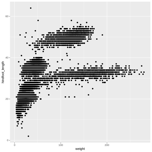
To add a geom to the plot use + operator. Because we
have two continuous variables, let’s use geom_point()
first:
R
ggplot(data = surveys_complete, aes(x = weight, y = hindfoot_length)) +
  geom_point()

The + in the ggplot2
package is particularly useful because it allows you to modify existing
ggplot objects. This means you can easily set up plot
“templates” and conveniently explore different types of plots, so the
above plot can also be generated with code like this:
R
# Assign plot to a variable
surveys_plot <- ggplot(data = surveys_complete,
                       mapping = aes(x = weight, y = hindfoot_length))

# Draw the plot
surveys_plot +
  geom_point()
Notes
- Anything you put in the
ggplot()function can be seen by any geom layers that you add (i.e., these are universal plot settings). This includes the x- and y-axis you set up inaes(). - You can also specify aesthetics for a given geom independently of
the aesthetics defined globally in the
ggplot()function. - The
+sign used to add layers must be placed at the end of each line containing a layer. If, instead, the+sign is added in the line before the other layer,ggplot2will not add the new layer and will return an error message. - You may notice that we sometimes reference ‘ggplot2’ and sometimes ‘ggplot’. To clarify, ‘ggplot2’ is the name of the most recent version of the package. However, any time we call the function itself, it’s just called ‘ggplot’.
- The previous version of the
ggplot2package, calledggplot, which also contained theggplot()function is now unsupported and has been removed from CRAN in order to reduce accidental installations and further confusion.
R
# This is the correct syntax for adding layers
surveys_plot +
  geom_point()

# This will not add the new layer and will return an error message
surveys_plot
  + geom_point()
Challenge (optional)
Scatter plots can be useful exploratory tools for small datasets. For
data sets with large numbers of observations, such as the
surveys_complete data set, overplotting of points can be a
limitation of scatter plots. One strategy for handling such settings is
to use hexagonal binning of observations. The plot space is tessellated
into hexagons. Each hexagon is assigned a color based on the number of
observations that fall within its boundaries. To use hexagonal binning
with ggplot2, first install the R package
hexbin from CRAN:
R
install.packages("hexbin")
Then use the geom_hex() function:
R
surveys_plot +
 geom_hex()
- What are the relative strengths and weaknesses of a hexagonal bin plot compared to a scatter plot? Examine the above scatter plot and compare it with the hexagonal bin plot that you created.
Building your plots iteratively
Building plots with ggplot2 is
typically an iterative process. We start by defining the dataset we’ll
use, lay out the axes, and choose a geom:
R
ggplot(data = surveys_complete, aes(x = weight, y = hindfoot_length)) +
    geom_point()
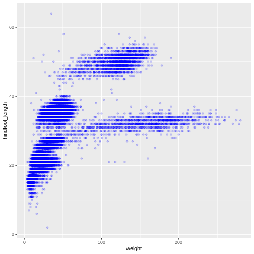
Then, we start modifying this plot to extract more information from
it. For instance, we can add transparency (alpha) to avoid
overplotting:
R
ggplot(data = surveys_complete, aes(x = weight, y = hindfoot_length)) +
    geom_point(alpha = 0.2)
We can also add colors for all the points:
R
ggplot(data = surveys_complete, mapping = aes(x = weight, y = hindfoot_length)) +
    geom_point(alpha = 0.2, color = "blue")
Adding another variable
Let’s try coloring our points according to the sampling plot type
(plot here refers to the physical area where rodents were sampled and
has nothing to do with making graphs). Since we’re now mapping a
variable (plot_type) to a component of the ggplot2 plot
(color), we need to put the argument inside
aes():
R
ggplot(data = surveys_complete, mapping = aes(x = weight, y = hindfoot_length)) +
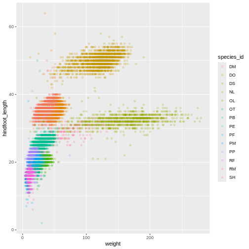
geom_point(alpha = 0.2, aes(color = species_id))
Challenge
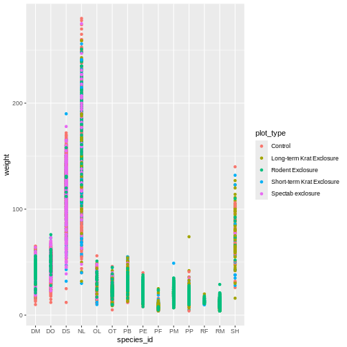
Use what you just learned to create a scatter plot of
weight over species_id with the plot types
showing in different colors. Is this a good way to show this type of
data?
R
ggplot(data = surveys_complete,
       mapping = aes(x = species_id, y = weight)) +
   geom_point(aes(color = plot_type))
Changing scales
The default discrete color scale isn’t always ideal: it isn’t
friendly to viewers with colorblindness and it doesn’t translate well to
grayscale. However, ggplot2 comes with
quite a few other color scales, including the fantastic
viridis scales, which are designed to be colorblind and
grayscale friendly. We can change scales by adding scale_
functions to our plots:
R
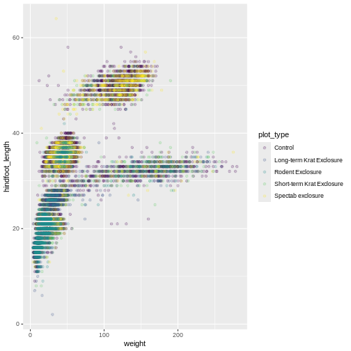
ggplot(data = surveys_complete, mapping = aes(x = weight, y = hindfoot_length, color = plot_type)) +
  geom_point(alpha = 0.2) +
  scale_color_viridis_d()
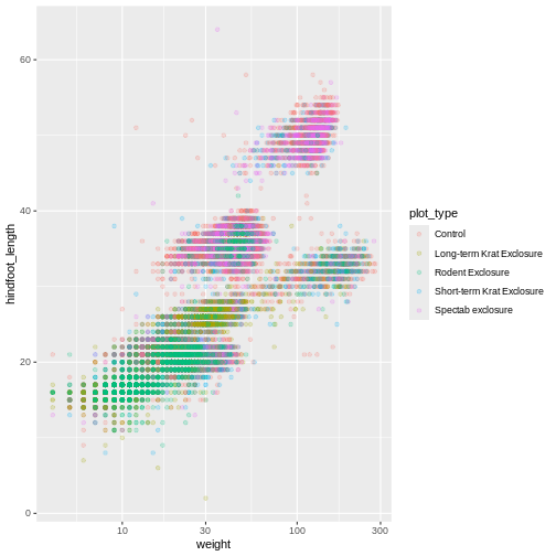
Scales don’t just apply to colors- any plot component that you put
inside aes() can be modified with scale_
functions. Just as we modified the scale used to map
plot_type to color, we can modify the way that
weight is mapped to the x axis by using the
scale_x_log10() function:
R
ggplot(data = surveys_complete, mapping = aes(x = weight, y = hindfoot_length, color = plot_type)) +
  geom_point(alpha = 0.2) +
  scale_x_log10()
One nice thing about ggplot and the
tidyverse in general is that groups of functions that do
similar things are given similar names. Any function that modifies a
ggplot scale starts with scale_, making it
easier to search for the right function.
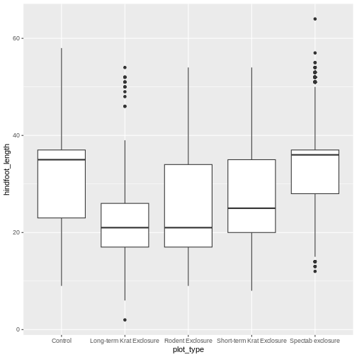
Boxplot
We can use boxplots to visualize the distribution of weight within each species:
R
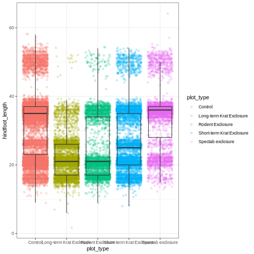
ggplot(data = surveys_complete, mapping = aes(x = plot_type, y = hindfoot_length)) +
  geom_boxplot()
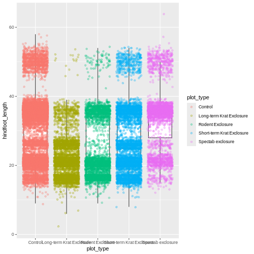
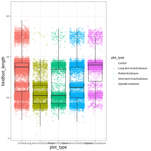
By adding points to the boxplot, we can have a better idea of the
number of measurements and of their distribution. Because the boxplot
will show the outliers by default these points will be plotted twice –
by geom_boxplot and geom_jitter. To avoid this
we must specify that no outliers should be added to the boxplot by
specifying outlier.shape = NA.
R
ggplot(data = surveys_complete, mapping = aes(x = plot_type, y = hindfoot_length)) +
  geom_boxplot(outlier.shape = NA) +
  geom_jitter(alpha = 0.3, aes(color = plot_type))
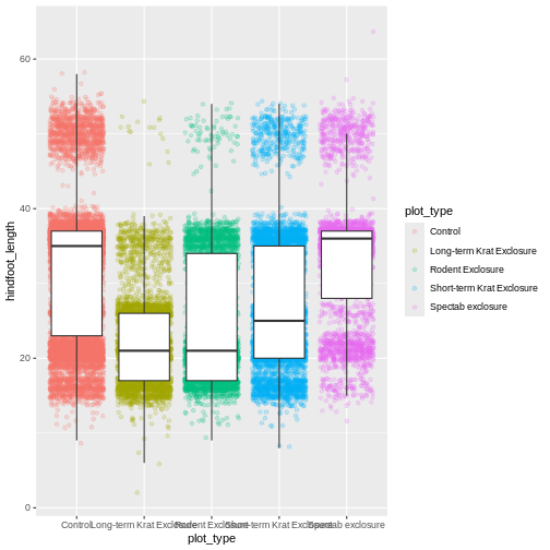
Now our points are colored according to plot_type, but
the boxplots are all the same color. One thing you might notice is that
even with alpha = 0.2, the points obscure parts of the
boxplot. This is because the geom_point() layer comes after
the geom_boxplot() layer, which means the points are
plotted on top of the boxes. To put the boxplots on top, we switch the
order of the layers:
R
ggplot(data = surveys_complete, mapping = aes(x = plot_type, y = hindfoot_length)) +
  geom_jitter(aes(color = plot_type), alpha = 0.2) +
  geom_boxplot(outlier.shape = NA)
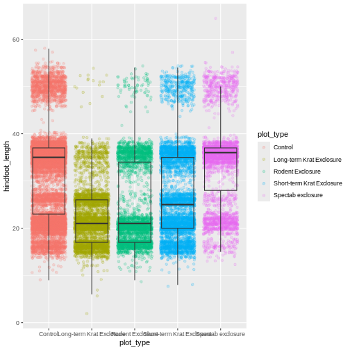
Now we have the opposite problem! The white fill of the
boxplots completely obscures some of the points. To address this
problem, we can remove the fill from the boxplots
altogether, leaving only the black lines. To do this, we set
fill to NA:
R
ggplot(data = surveys_complete, mapping = aes(x = plot_type, y = hindfoot_length)) +
  geom_jitter(aes(color = plot_type), alpha = 0.2) +
  geom_boxplot(outlier.shape = NA, fill = NA)

Now we can see all the raw data and our boxplots on top.
Changing themes
So far we’ve been changing the appearance of parts of our plot
related to our data and the geom_ functions, but we can
also change many of the non-data components of our plot.
At this point, we are pretty happy with the basic layout of our plot,
so we can assign it to a plot to a named
object. We do this using the assignment
arrow <-. What we are doing here is taking the
result of the code on the right side of the arrow, and assigning it to
an object whose name is on the left side of the arrow.
We will create an object called myplot. If you run the
name of the ggplot2 object, it will show the plot, just
like if you ran the code itself.
R
myplot <- ggplot(data = surveys_complete, mapping = aes(x = plot_type, y = hindfoot_length)) +
  geom_jitter(aes(color = plot_type), alpha = 0.2) +
  geom_boxplot(outlier.shape = NA, fill = NA)

myplot
This process of assigning something to an object is
not specific to ggplot2, but rather a general feature of R.
We will be using it a lot in the rest of this lesson. We can now work
with the myplot object as if it was a block of
ggplot2 code, which means we can use + to add
new components to it.
We can change the overall appearance using theme_
functions. Let’s try a black-and-white theme by adding
theme_bw() to our plot:
R
myplot + theme_bw()
As you can see, a number of parts of the plot have changed.
theme_ functions usually control many aspects of a plot’s
appearance all at once, for the sake of convenience. To individually
change parts of a plot, we can use the theme() function,
which can take many different arguments to change things about the text,
grid lines, background color, and more. Let’s try changing the size of
the text on our axis titles. We can do this by specifying that the
axis.title should be an element_text() with
size set to 14.
R
myplot +
  theme_bw() +
  theme(axis.title = element_text(size = 14))
Another change we might want to make is to remove the vertical grid
lines. Since our x axis is categorical, those grid lines aren’t useful.
To do this, inside theme(), we will change the
panel.grid.major.x to an element_blank().
R
myplot +
  theme_bw() +
  theme(axis.title = element_text(size = 14),
        panel.grid.major.x = element_blank())
Another useful change might be to remove the color legend, since that
information is already on our x axis. For this one, we will set
legend.position to “none”.
R
myplot +
  theme_bw() +
  theme(axis.title = element_text(size = 14),
        panel.grid.major.x = element_blank(),
        legend.position = "none")
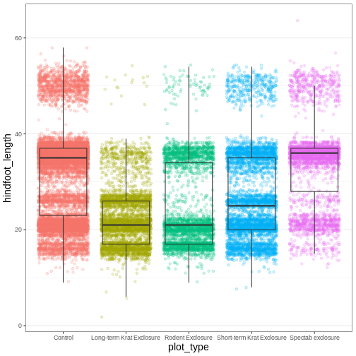
Because there are so many possible arguments to the
theme() function, it can sometimes be hard to find the
right one. Here are some tips for figuring out how to modify a plot
element:
- type out
theme(), put your cursor between the parentheses, and hit Tab to bring up a list of arguments- you can scroll through the arguments, or start typing, which will shorten the list of potential matches
- like many things in the
tidyverse, similar argument start with similar names- there are
axis,legend,panel,plot, andstriparguments
- there are
- arguments have hierarchy
-
textcontrols all text in the whole plot -
axis.titlecontrols the text for the axis titles -
axis.title.xcontrols the text for the x axis title
-
You may have noticed that we have used 3 different approaches to
getting rid of something in ggplot:
-
outlier.shape = NAto remove the outliers from our boxplot -
panel.grid.major.x = element_blank()to remove the x grid lines -
legend.position = "none"to remove our legend
Why are there so many ways to do what seems like the same thing?? This is a common frustration when working with R, or with any programming language. There are a couple reasons for it:
- Different people contribute to different packages and functions, and they may choose to do things differently.
- Code may appear to be doing the same thing, when the
details are actually quite different. The inner workings of
ggplot2are actually quite complex, since it turns out making plots is a very complicated process! Because of this, things that seem the same (removing parts of a plot), may actually be operating on very different components or stages of the final plot. - Developing packages is a highly iterative process, and sometimes
things change. However, changing too much stuff can make old code break.
Let’s say removing the legend was introduced as a feature of
ggplot2, and then a lot of time passed before someone added the feature letting you remove outliers fromgeom_boxplot(). Changing the way you remove the legend, so that it’s the same as the boxplot approach, could break all of the code written in the meantime, so developers may opt to keep the old approach in place.
Changing labels
Our plot is really shaping up now. However, we probably want to make
our axis titles nicer, and perhaps add a main title to the plot. We can
do this using the labs() function:
R
myplot +
  theme_bw() +
  theme(axis.title = element_text(size = 14),
        legend.position = "none") +
  labs(title = "Rodent size by plot type",
       x = "Plot type",
       y = "Hindfoot length (mm)")
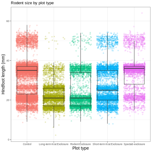
We removed our legend from this plot, but you can also change the
titles of various legends using labs(). For example,
labs(color = "Plot type") would change the title of a color
scale legend to “Plot type”.
Challenge 3: Customizing a plot
Modify the previous plot by adding a descriptive subtitle. Increase the font size of the plot title and make it bold.
Hint: “bold” is referred to as a font “face”
R
myplot +
  theme_bw() +
  theme(axis.title = element_text(size = 14), legend.position = "none",
        plot.title = element_text(face = "bold", size = 20)) +
  labs(title = "Rodent size by plot type",
       subtitle = "Long-term dataset from Portal, AZ",
       x = "Plot type",
       y = "Hindfoot length (mm)")
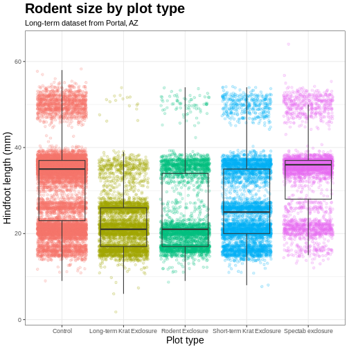
Faceting
One of the most powerful features of
ggplot is the ability to quickly split a
plot into multiple smaller plots based on a categorical variable, which
is called faceting.
So far we’ve mapped variables to the x axis, the y axis, and color, but trying to add a 4th variable becomes difficult. Changing the shape of a point might work, but only for very few categories, and even then, it can be hard to tell the differences between the shapes of small points.
Instead of cramming one more variable into a single plot, we will use
the facet_wrap() function to generate a series of smaller
plots, split out by sex. We also use ncol to
specify that we want them arranged in a single column:
R
myplot +
  theme_bw() +
  theme(axis.title = element_text(size = 14),
        legend.position = "none",
        panel.grid.major.x = element_blank()) +
  labs(title = "Rodent size by plot type",
       x = "Plot type",
       y = "Hindfoot length (mm)",
       color = "Plot type") +
  facet_wrap(vars(sex), ncol = 1)
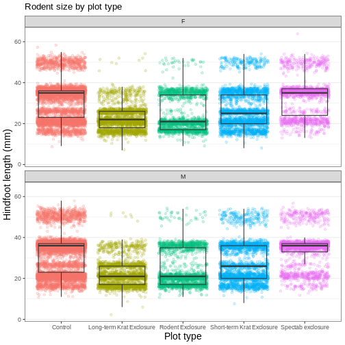
Faceting comes in handy in many scenarios. It can be useful when:
- a categorical variable has too many levels to differentiate by color (such as a dataset with 20 countries)
- your data overlap heavily, obscuring categories
- you want to show more than 3 variables at once
- you want to see each category in isolation while allowing for general comparisons between categories
Exporting plots
Once we are happy with our final plot, we can assign the whole thing
to a new object, which we can call finalplot.
R
finalplot <- myplot +
  theme_bw() +
  theme(axis.title = element_text(size = 14),
        legend.position = "none",
        panel.grid.major.x = element_blank()) +
  labs(title = "Rodent size by plot type",
       x = "Plot type",
       y = "Hindfoot length (mm)",
       color = "Plot type") +
  facet_wrap(vars(sex), ncol = 1)
After this, we can run ggsave() to save our plot. The
first argument we give is the path to the file we want to save,
including the correct file extension. This code will make an image
called rodent_size_plots.jpg in the fig/
folder of our current project. We are making a .png, but
you can save .pdf, .tiff, and other file
formats. Next, we tell it the name of the plot object we want to save.
We can also specify things like the width and height of the plot in
inches.
R
ggsave(filename = "fig/rodent_size_plots.png", plot = finalplot,
       height = 6, width = 8)
Challenge 4: Make your own plot
Try making your own plot! You can run
glimpse(surveys_complete) to explore variables you might
use in your new plot. Feel free to use variables we have already seen,
or some we haven’t explored yet.
Here are a couple ideas to get you started:
- make a histogram of one of the numeric variables
- try using a different color
scale_ - try changing the size of points or thickness of lines in a
geom
- the
ggplot()function initiates a plot, andgeom_functions add representations of your data - use
aes()when mapping a variable from the data to a part of the plot - use
scale_functions to modify the scales used to represent variables - use premade
theme_functions to broadly change appearance, and thetheme()function to fine-tune - start simple and build your plots iteratively